


Disclaimer. This is educational research, not financial advice. Every performance number below comes from simulated backtests or from a model, not from live trading. Futures and options can lose more than you put in. Do your own work and talk to a qualified adviser before trading.
Every word, chart, payoff diagram and line of code in this article was produced by AI agents. Behind the scenes, this publication now runs on AI agents end to end. They read the raw bot reports and backtests, price the options structures, write and benchmark the C++, and build the post itself, and I keep only the final sign-off on anything that goes live, spends money or touches a real trading account. I explain why I chose this stack in Why I'm Choosing Grok Bot with Cursor for AI Coding Agents. In short, it's an agent that works inside a real IDE, against a maintained repository, and plugs straight into the platforms the business runs on. This piece shows what that stack can do when you point it at five live futures bots and seven research PDFs with no prior context, and it's only the beginning. Expect more research, more tools and more autonomous workflows like this here at theorderbookedge.com and over at hftcode.com.
On Monday, November 9, 2026, at 3:01 PM ET, my research pipeline wrote a fresh report folder with seven PDFs. One is a 24-page institutional narrative covering futures and options-on-futures. The rest cover five micro-futures trading bots: a backtest term sheet, a live dashboard, a portfolio summary, a risk-protocol reference, an options-chain overlay and a signal-integration report. This article starts from those seven files and nothing else. I didn’t carry over any earlier rankings, conclusions or templates.
I set myself three jobs:
Find the most profitable institutional options and futures structures that the documents actually support, and price each one with real payoff math.
Audit the five bots the way a risk committee would, covering performance, drawdown, Sharpe, statistical significance and leverage, and decide which ones deserve capital.
Hand you the toolkit: the equations, the Python and four ultra-low-latency C++ programs that I compiled and ran while writing this.
One rule held throughout. The bots’ trading rules are proprietary, so I describe them only at the level of “trend-following with a macro filter” and never give the parameters. The analysis doesn’t need them anyway.
The short version
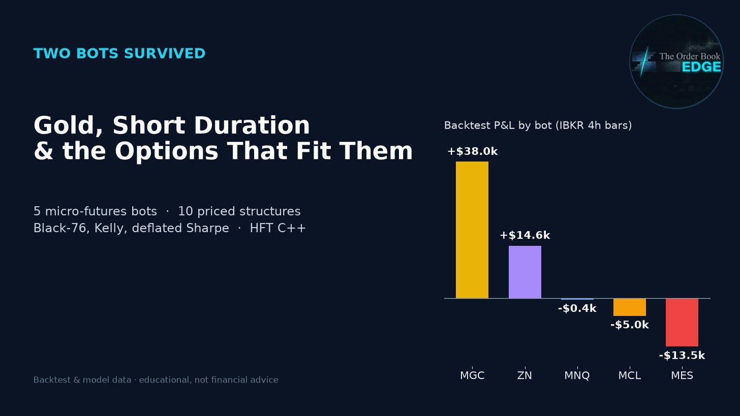
Two of the five bots made money in backtest. Micro Gold Safe Haven (long MGC) made +$38,029 on 67 trades: 34 wins, 33 losses, a 50.7% win rate, profit factor 1.79 and Sharpe 2.12. Micro 10Y Treasury Yield Curve (short ZN) made +$14,609 on 12 trades: 6 wins, 6 losses, profit factor 1.77 and Sharpe 0.88. The other three lost money: Nasdaq trend ‑$415, crude momentum ‑$4,989 and S&P breakout ‑$13,540. All five together made +$33,694.
The planner was badly overconfident. The AI planner projected Sharpe ratios of 1.5 to 1.9 for every bot. The backtests averaged 0.17.
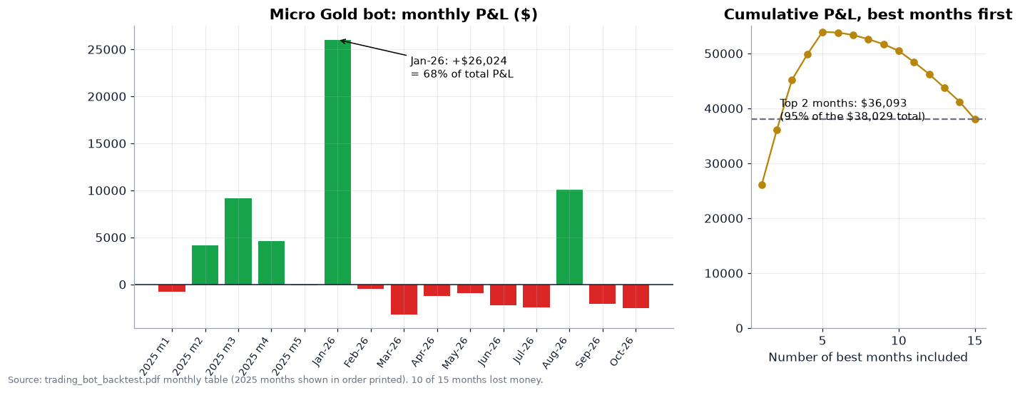
The gold bot’s edge is real but fragile. One month, January 2026, produced 68% of its P&L, and its best two months produced 95%. Ten of its fifteen months lost money. Its per-trade t-stat is 2.32. Once you deflate for the fact that five bots were tested, the probability that the Sharpe is genuinely positive falls from about 99% to about 60%.
The headline drawdowns are mis-scaled. The “91.6%” and “99.8%” figures divide by starting capital. Measured against peak equity, the Treasury bot’s worst drawdown was 33.6% and the gold bot’s was about 24% or less. Both still break the system’s own 20% limit.
“Micro 10Y” is really a full-size Treasury note position. The bot’s P&L reconciles to a $1,000-per-point multiplier on five contracts, about $540,000 of notional on $15,000 of capital (36x). The PDF prints “1000x leverage” for every bot. That line is a placeholder bug.
No live data reached the bots in this run. There were zero live trades, zero of five bots received market data, zero options strikes came back with Greeks and zero integration signals fired. Everything below is backtest or model output.
The best risk-adjusted structures follow the two surviving bots. A gold 4100/4300 call debit spread costs $5,235, has a $14,740 maximum gain and a 2.80 reward-to-risk ratio. A zero-cost gold spread collar pairs a short 3900/3700 put spread with a long 4200/4400 call spread. A ZN 108/106 put spread costs $832 with a $1,164 maximum gain. For tails, an ES 7000/6800 put spread costs $206 and pays up to $9,793 (47 to 1), and a VIX 25/30 call spread pays 4.7 to 1. I’d avoid two things. The report’s own Treasury hedge (short ZN plus a 110/115 call spread) leaves the loss open-ended above 115. The NatGas short strangle wins 69% of the time but has open-ended losses.
Even a tenth of Kelly is about as far as this edge stretches. I simulated the gold edge at full, half, quarter and one-tenth Kelly. Only around one-tenth Kelly keeps the median drawdown under the 20% rule. Coincidentally, that is roughly what the PDF’s “risk 1-2% per trade” rule implies.
Everything after the break is the full working: sixteen data-integrity bugs, every payoff diagram, the macro drivers, and copy-paste Python and C++.
1. What the seven PDFs actually contain
Before you trust a number, you need to know where it came from. The run produced a narrative report first (15:01 ET) and then six bot documents about eighteen minutes later. The narrative was written from the day’s news flow. The bot documents come from a one-year backtest on IBKR four-hour bars, plus a live dashboard that, for this run, never received data.

The most important line is the health column. The dashboard shows 5 bots, 0 bots with trades, 0 total trades, 407 rules enforced and $0.00 combined P&L. It reports “NO POLLING DATA”, 0% data success and 0 of 5 bots receiving data. The options-chain overlay returned symbol ESM26 with a futures mid of 0.00, 25 “clean quotes”, 84 total open interest and zero strikes with live Greeks. The signal overlay found 0 signals, with a news-sentiment multiplier of exactly 1.0000x.
So none of this run’s live analytics, meaning options Greeks, IV surface, skew and signal relevance, contain real data. The quantitative evidence is the backtest. The narrative report supplies themes, and as you’ll see, its price levels aren’t reliable. I’ve built the article around that: backtests for the bots, the report for direction and drivers, and Black-76 with clearly labelled inputs wherever a price is needed.
2. The macro tape: the institutional drivers behind the formulas
The report covers seven asset complexes and repeats itself in four overlapping passes. Here are the themes that recur in at least three passes. These are the drivers that justify the formulas later on. Treat every specific number in this section as cited by the report, not checked against exchange data.
2.1 Rates: higher for longer, with a hawkish tail
This is the strongest thread in the document. It cites:
an October payrolls beat of +165K against roughly 59K to 65K expected, with unemployment at 4.1%;
ISM services and manufacturing both above 50;
a CME FedWatch probability of 76% for a 25 bp December hike, up from about 50% a week earlier.
Positioning reinforces it. CTA funds are described as running a net short of 450K contracts in 10-year note futures, called “extreme” and “record”. The report also describes a weak 30-year auction, the SOFR one-year mid-curve CVOL at 137.79 (its highest since late summer), and 5y5y breakeven inflation moving from 2.2% to 2.4% in a month.
The curve story is less consistent. The report quotes 2s10s at both ‑30 bp and ‑50 bp, and recommends both steepeners and flatteners in different sections. The direction, though, is consistent: front-end yields up, duration under pressure. The Treasury bot’s trade log independently confirms it. ZN futures fell from about 113.9 in late June to 102.8 in mid-October before bouncing to about 108.
Formula consequence: a short-duration view fits a put spread on ZN better than outright shorts. Implied vol has already risen (12% vs 10% a month ago, as cited), so a spread lets you sell back some of that richness. CPI on November 10 and the FOMC on December 15 are two jump events inside the 38-day window, which argues for paying for convexity rather than selling it.
2.2 Energy: two-way risk premium, structural freight tightness
Oil is pulled in both directions:
Bearish: a possible Hormuz reopening deal (Brent cited as falling 3.6% to $94) and OPEC+ output back to 90% of pre-war levels.
Bullish: a Saudi pipeline attack, Ukrainian strikes on Russian refineries and a structural freight story. The report says VLCC freight is running at 25-30% of delivered oil cost against 3-5% historically, with no new VLCC orders before 2030.
The spread signals are the cleanest. The Brent-WTI premium is cited as widening from $3.00 to $4.50, and CLZ6-CLZ7 as flipping to +$1.20 backwardation. OVX is cited at 45% and WTI option IV at 35% (from 30%).
Formula consequence: with high implied vol and two-way headline risk, debit spreads (defined risk, vega partly hedged) beat naked options. The one recommendation I can’t support is the report’s short NatGas strangle, discussed below. NG IV is quoted at 60%+ after a short squeeze, which looks like a premium-selling opportunity but is exactly the kind of tail that ruins short-vol books.
2.3 Gold: safe haven vs. real yields
The report frames gold as “decoupling from rates”, supported by central-bank buying and geopolitical tails. It also cites strong negative correlations: gold vs DXY at about ‑0.8 and gold vs real yields at about ‑0.75. That tension matters for the portfolio. Long gold and short Treasury notes are partial hedges for each other. When real yields jump, the ZN short gains while gold falls, and vice versa. Our two surviving bots happen to be structurally diversified.
The price levels are another matter. The report quotes gold at $1,920 with strikes from 1,800 to 2,300. The gold bot’s trade log has gold trading between about $4,050 and $5,577 over 2026. Those can’t both describe the same market. I therefore map the report’s structures by moneyness onto the trade-log price (about $4,050) and label every gold strike in this article as mapped.
2.4 Equity indices and volatility: hedged longs into CPI
The report describes hedge funds and CTAs as long ES and NQ, with heavy put buying ahead of CPI. It cites ES IV rising from 12% to 14%, NQ from 15% to 18%, VXN at 39 and a 4.5% single-day drop described as the largest of 2026. Its VIX regime table ties position size to VIX. Below 15 means full size, 15-25 means cut 25%, 25-35 means cut 50%, and above 35 means cut 75%.
But the same report reads VIX at “<15”, “~22” and “>25” in different sections, which would put the same day in three different sizing buckets. I chart that below. It’s a good example of why a sizing rule needs one authoritative data feed.
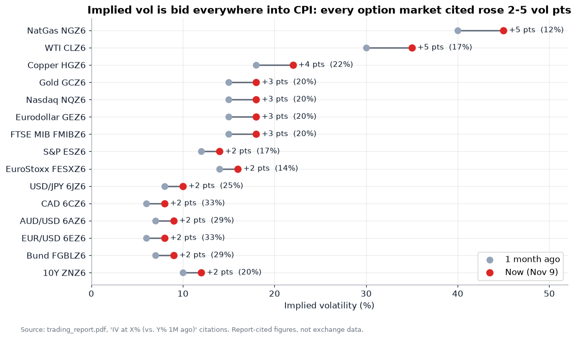
Every options market the report cites shows implied vol up 2 to 5 points in a month. Proportionally, the biggest increases are in FX (EUR, CAD, AUD and JPY up 25-33%). The biggest absolute increases are in NatGas and WTI (+5 points each). That’s a market paying up for event protection into CPI, which is why I favour spreads over outright long options throughout.
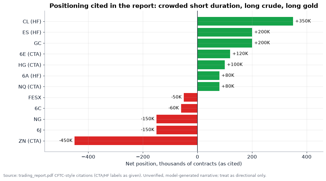
The positioning picture is crowded short duration, crowded long crude and long gold, and short yen and CAD futures. Crowding is a driver in itself. A hawkish surprise is partly priced into a 450K-contract short, so the asymmetric risk for ZN shorts is a short squeeze on a soft CPI. That’s another argument for defined-risk put spreads over outright futures shorts.
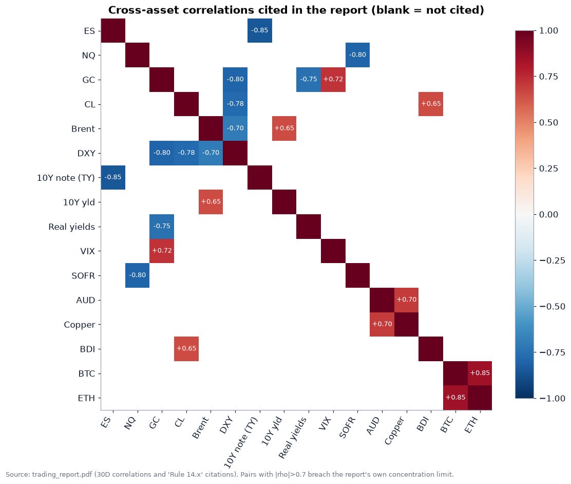
The report applies its own rule to these correlations: avoid stacking positions whose pairwise correlation exceeds 0.7. Several cited pairs exceed it: ES vs 10-year note futures at ‑0.85, NQ vs SOFR at ‑0.80, gold vs DXY at ‑0.80, and CL vs DXY at ‑0.78. In practice the USD, Treasuries and oil behave like one macro factor here. If you hold the ZN short, an extra DXY long adds little diversification.
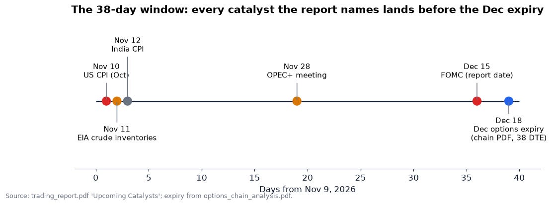
The calendar argues for buying convexity. US CPI (Nov 10), EIA inventories (Nov 11), India CPI (Nov 12), OPEC+ (Nov 28) and the FOMC (Dec 15) all fall before the December 18 expiry that the chain PDF references, 38 days out. Every option structure below is priced to that 38-day horizon.
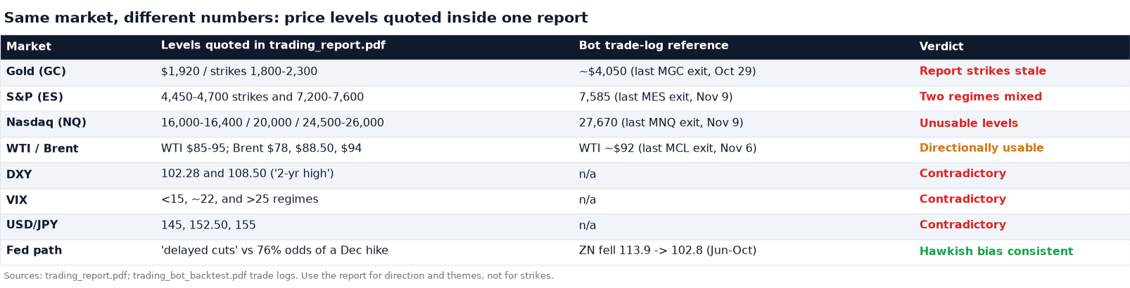
Finally, the caveat that shapes everything else. Inside one 24-page document, ES appears at both 4,500 and 7,500, NQ at 16,000, 20,000 and 25,000 against a trade log at 27,670, DXY at both 102 and 108.5, and USD/JPY at 145, 152.5 and 155. The report also recommends trades in Eurodollar futures and options, a contract family CME converted to SOFR in 2023. The narrative reads like a model synthesizing several news snapshots. It’s useful for what institutions care about, but not for where prices are. Wherever a level matters, I use the bots’ trade logs.
3. The five bots: a risk-committee audit
All five bots trade CME-group micro futures (or are labelled that way), one contract family each. Their logic is described conceptually as trend-following or momentum with a macro-theme filter taken from the narrative report. The backtest uses IBKR four-hour bars. The data windows run from about seven months (ZN) to about two years (MCL), even though every PDF calls them “1-year”. Starting capital is $12,000 to $18,000 per bot, $75,000 in total.

Here are the wins, losses and win/loss ratios in full, along with average and largest trades and streaks:

3.1 Projection vs reality
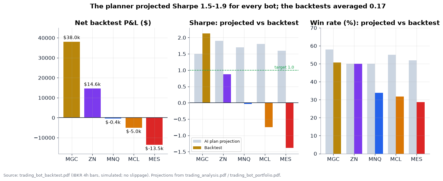
The AI planner that designed these bots projected annual returns of 30-45%, Sharpe ratios of 1.5-1.9 and win rates of 50-58% for every bot, and it labelled all five “expected” to work. The backtests produced three losers and an average Sharpe of 0.17. The gap between projected and realized Sharpe ranges from +0.62 (gold beat its projection) to ‑2.98 (MES). The lesson isn’t that the planner is useless. Its macro themes picked the two directions that worked: long gold, short duration. But its risk numbers are priors, not estimates, and they shouldn’t be anywhere near a sizing formula.
3.2 One payoff shape, five win rates
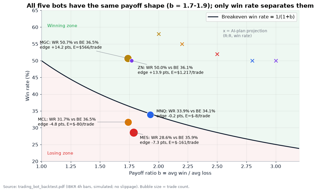
This is the most useful single chart in the bot section. Every bot has nearly the same payoff ratio b = average win / average loss, between 1.74 and 1.93. That’s the signature of a shared exit architecture: a profit target set as a multiple of the stop distance. When b is fixed, the breakeven win rate is fixed too:
breakeven win rate p* = 1 / (1 + b) b = 1.74 -> p* = 36.5%
So the whole question becomes whether the entry signal can beat a ~36% hit rate on that market:
Gold clears it by 14.2 points, with an expectancy of about +$566 per trade.
ZN clears it by 13.9 points, about +$1,217 per trade.
MNQ misses by 0.2 points. Profit factor 0.99 is a coin flip that pays its costs.
MCL misses by 4.8 points and MES by 7.3 points.
The ✕ markers show the planner’s projected (R:R, win rate) pairs. They all sit in the green zone, well away from where the bots actually landed. For a momentum system, entry quality is the strategy, so the bots that failed failed because their markets didn’t trend in the four-hour bars.
3.3 Micro Gold Safe Haven: the winner with a concentration problem
On the headline numbers, gold is excellent: +$38,029 on $15,000, Sharpe 2.12, Sortino 7.39, Calmar 2.77 and a composite grade of B+. The monthly table changes the picture:
January 2026 alone made +$26,024, 68% of all P&L. January plus August 2026 (+$10,069) made $36,093, or 95%.
Ten of fifteen months lost money. From February to July 2026 the bot gave back $10,429 in six straight losing months.
Its last 20 trades netted ‑$5,682, with 6 winners. Gold slid from about $5,577 to about $4,090 between March and late October 2026, and a long-only trend bot bleeds in a falling market.
A Sortino of 7.39 can coexist with a 33% profitable-month rate because a few huge right-tail months dominate the denominator. That’s fine if you believe the right tail will recur, and dangerous if January 2026 was a one-off regime. The forward “Probability of Profit: 94%” in the PDF is not a forecast. It’s a transformation of in-sample win rate and profit factor, and the significance test below cuts it down hard.
There’s also a stale-parameter issue that I’ll describe without giving the parameter. The strategy description references a gold price level far below where gold traded for the whole backtest. If the live code matches the description, that filter is always on, so the bot is effectively unconditionally long whenever its trend condition fires. That may be harmless. It still needs checking.
Verdict: viable, at small size, with a regime kill-switch. The edge is statistically detectable on its own (t ≈ 2.3), but it’s concentrated, and the recent tape is against it.
3.4 Micro 10Y Treasury Yield Curve: right thesis, tiny sample
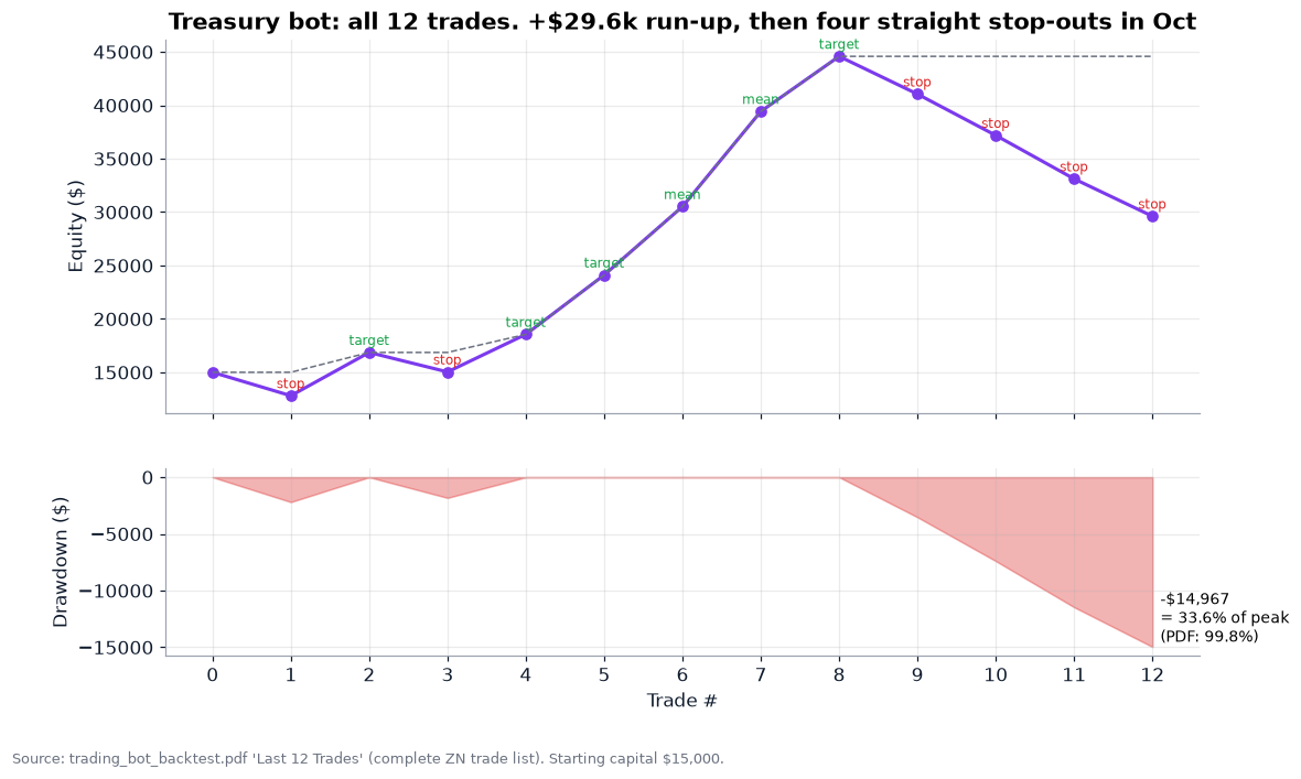
The ZN bot is the only one whose entire trade list is printed, so I could rebuild its equity curve exactly. Four of the first eight trades hit their target and two exited on a mean-reversion rule. The run reached +$29,576. Then October 15-30 produced four straight stop-outs totalling ‑$14,966. That’s the whole drawdown, inside about two weeks, as ZN bounced from 102.8 to 108.
The PDF prints the drawdown as 99.8%. Against peak equity of $44,576, it’s 33.6%. That’s still too much for a 20% rule, but it isn’t a near-wipeout. The ~159% “annual return” is about 97% earned in roughly four trading months and simple-annualised.
Three issues matter more than the drawdown:
Sample size. Twelve trades give a per-trade t-stat of 0.96. That’s indistinguishable from luck, and two good months (August and September) made the whole result.
Contract identity. The bot is called “Micro 10Y”, but the P&L reconciles to a $1,000-per-point multiplier, the full-size 10-year note. The IBKR contract field says ZBZ6, which is the 30-year bond. Five full ZN contracts is about $540,000 notional on $15,000 (36x). That leverage explains both the size of the winners and the speed of the October drawdown.
Crowding. The thesis is the same one the report says CTAs are already 450K contracts short. When everyone is short duration, the left tail is a squeeze. That’s what October looked like.
Verdict: the thesis is supported by the macro narrative and by price action, but the evidence for this bot’s edge is weak. Run it at a fraction of the size, preferably through defined-risk options (Section 4).
3.5 The three losers
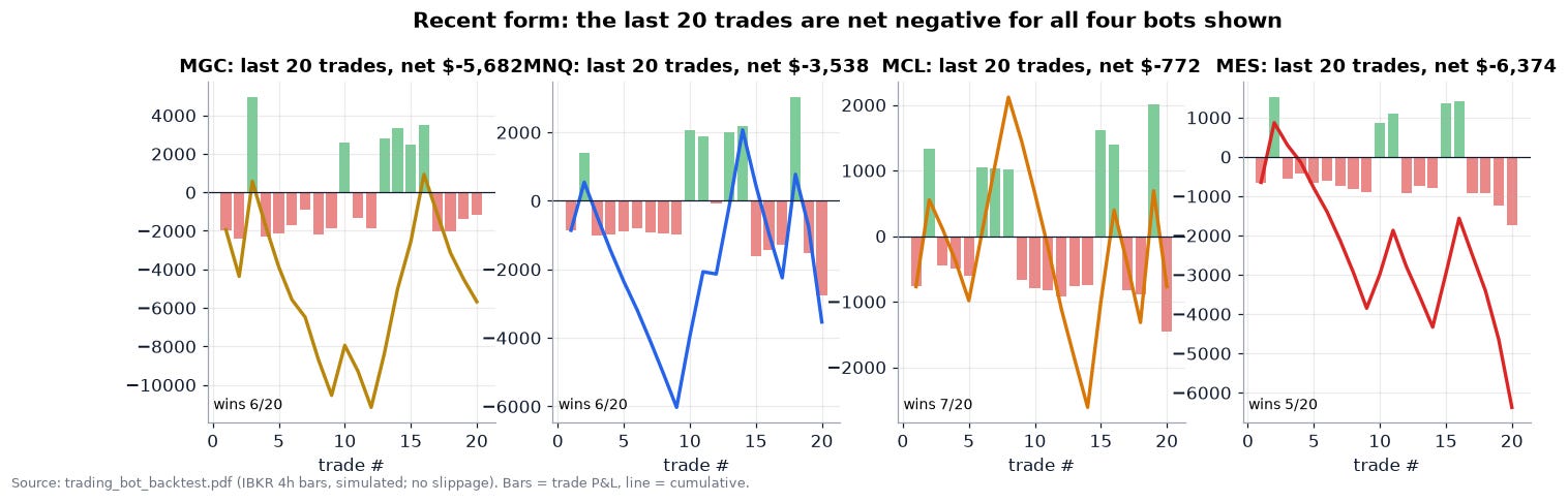
MNQ trend follower (‑$415, PF 0.99, Sharpe ‑0.03). It sits right on the breakeven frontier. Its 56 trades include a ‑$7,485 month and a +$6,022 month, so the volatility is real and the edge isn’t. The PDF calls it “MARGINAL” and suggests tightening entries. I’d keep it in paper trading only. With a payoff ratio of 1.93 it needs just a 34.1% hit rate, so a better entry filter could flip it. That’s an experiment, not an allocation.
MCL crude momentum (‑$4,989, PF 0.81, Sharpe ‑0.75). It lost in 9 of 14 months, mostly in small amounts, which is what death by whipsaw looks like in a headline-driven, range-bound oil market. That’s exactly the two-way-risk regime described in Section 2.2. Off.
MES breakout (‑$13,540, PF 0.72, Sharpe ‑1.38). This is the worst performer: a 28.6% win rate, seven straight losses at its worst, and a $16,818 drawdown that exceeds its $15,000 starting capital (112%). The PDF diagnoses “REGIME_COLLAPSE”: profitable early, then breaking down as the index chopped between about 7,470 and 7,870 in its final 20 trades. The same document also says “IBKR unavailable: Rithmic Ticker Plant login failed, using plan metrics”, yet prints a full trade log. Its data provenance is uncertain. Off, and quarantined until the data question is answered.
3.6 Restating drawdown and leverage
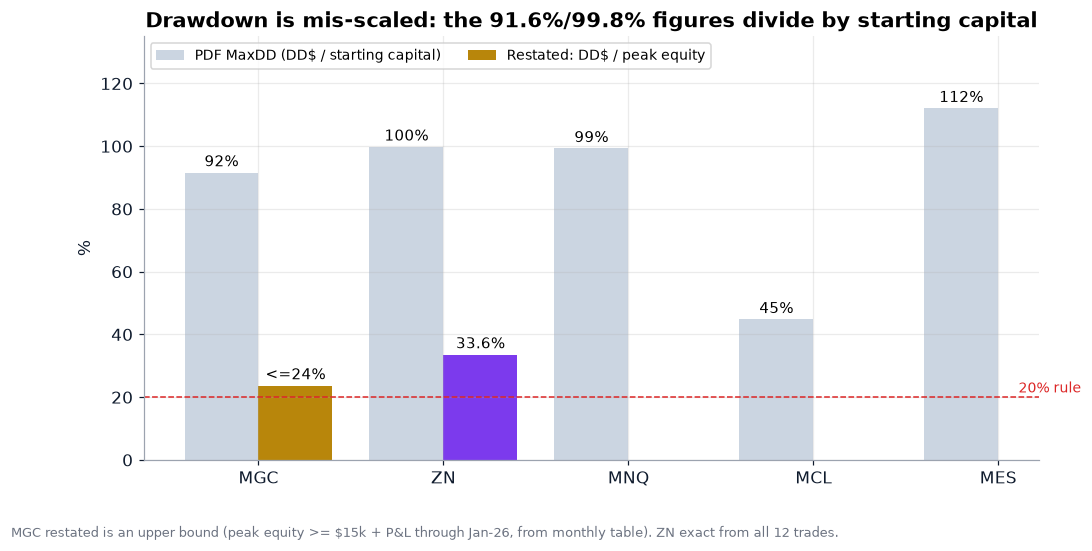
Every MaxDD % in the PDFs is drawdown dollars divided by starting capital. That’s a legitimate “how close did I get to ruin if the drawdown came first” measure, but it isn’t the standard definition, and it makes the profitable bots look catastrophic. Restated against peak equity, ZN is 33.6% (exact) and gold is at most about 24%. Both still breach the 20% target, so the conclusion is the same, but for the right reason.

The capital tables show a “Last Close Price” of $1e+05 for gold and $2,200 for ZN, notionals of $0.6M-$2.2M per contract and “Notional leverage: 1000.0x” for every bot. Those are placeholders: the margin figure multiplied by a constant. Using the last trade-log price and each contract’s multiplier, real exposure ranges from 2.0x (MCL) to 36x (ZN), with gold at 8.1x and the equity-index bots at 7.6x-9.2x.
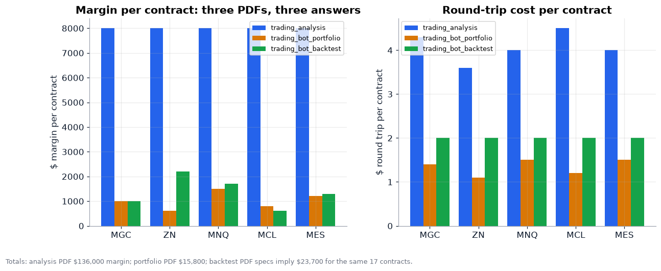
The documents also disagree about costs. For the same 17 contracts, the analysis PDF assumes $8,000 of margin per contract ($136,000 total), the portfolio PDF $600-$1,500 ($15,800 total), and the backtest PDF $600-$2,200 ($23,700 total). Round-trip costs range from $1.10 to $4.50 per contract depending on the document. At the backtest’s $2.00 round trip, costs are a rounding error against average trades of $600-$5,600. Margin is a different matter, because it decides how many lots fit in the account. Use your broker’s live numbers.
3.7 Is any of it statistically real?
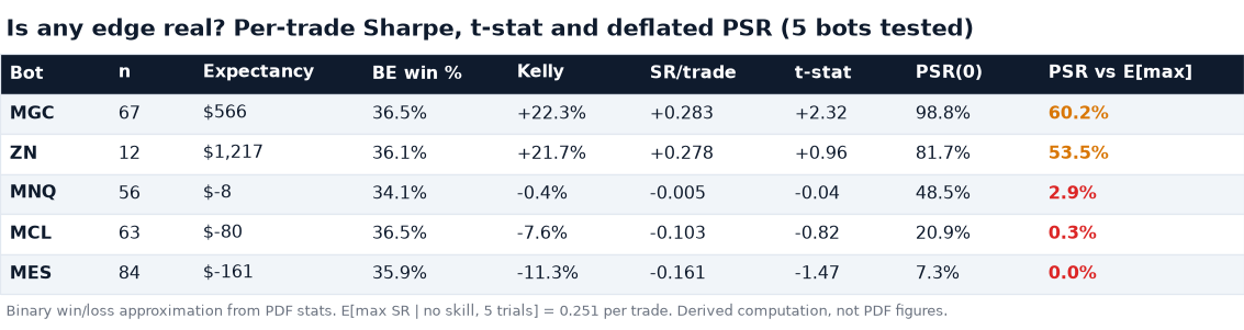
Here’s the test the PDFs leave out. Treat each trade as a draw. The per-trade Sharpe is expectancy divided by the standard deviation of trade P&L. The Probabilistic Sharpe Ratio (PSR) is the probability that the true Sharpe exceeds a benchmark, given sample length, skew and kurtosis. Against a benchmark of zero:
Gold: PSR 98.8% (t = 2.32)
ZN: 81.7% (t = 0.96)
MNQ: 48.5%
MCL: 20.9%
MES: 7.3%
But we tested five bots and picked the best. Under the False Strategy Theorem, the expected maximum per-trade Sharpe among five skill-less strategies with this cross-sectional dispersion is about 0.251. Use that as the benchmark (the deflated PSR) and gold falls to 60.2% and ZN to 53.5%. In plain English: allowing for selection bias, the best bot is a little better than a coin flip to have real skill. That’s not a reason to discard it. It is a reason to size it like a hypothesis rather than a certainty.
Bot verdicts:

4. Ranking the institutional options-on-futures structures
The report names more than 60 options trades. I shortlisted the ten that appear in its “final trade ideas” tables or recur in several passes, and that can be priced coherently. Each one is priced with Black-76 using the following inputs:
the last trade-log price as the underlying (gold 4,050.40, ZN 107.95, WTI 92.19, ES 7,585.12);
the report’s cited implied vol (gold 18%, ZN 12%, WTI 35%, ES 14%, NG 60%);
38 days to expiry and a 4.5% rate (the report’s SOFR pricing).
Where the PDFs give no usable input, I’ve marked the assumption with an asterisk: the VIX futures level and its vol, BTC level and vol, and the NG level. I use flat vol (no skew), so each figure is a model price, not a quote. Dollar figures are per standard contract. Divide by ten for micros (MGC, MCL, MES).
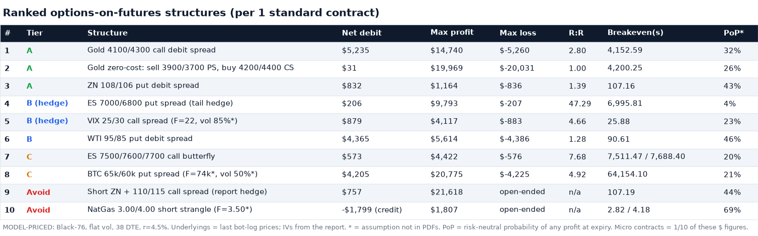
How I ranked them. Under the pricing measure, every structure’s expected P&L is zero by construction. My engine computes the risk-neutral EV of each one, and all ten come out at $0 to within a dollar. Nothing here is “free money”. The profit has to come from one of three places:
A directional view with evidence behind it. Only two exist in this run: long gold and short duration, from the two profitable bots plus the macro narrative.
A vol risk premium, where implied vol is above what will be realized.
Convexity bought cheaply before catalysts.
So the ranking is by evidence alignment first, then reward-to-risk and defined risk. Tier A structures express a view the backtests support. Tier B are hedges, or report views with no backtest behind them. Tier C are speculative. “Avoid” means open-ended risk or a structural flaw.
4.1 Tier A #1: gold 4100/4300 call debit spread
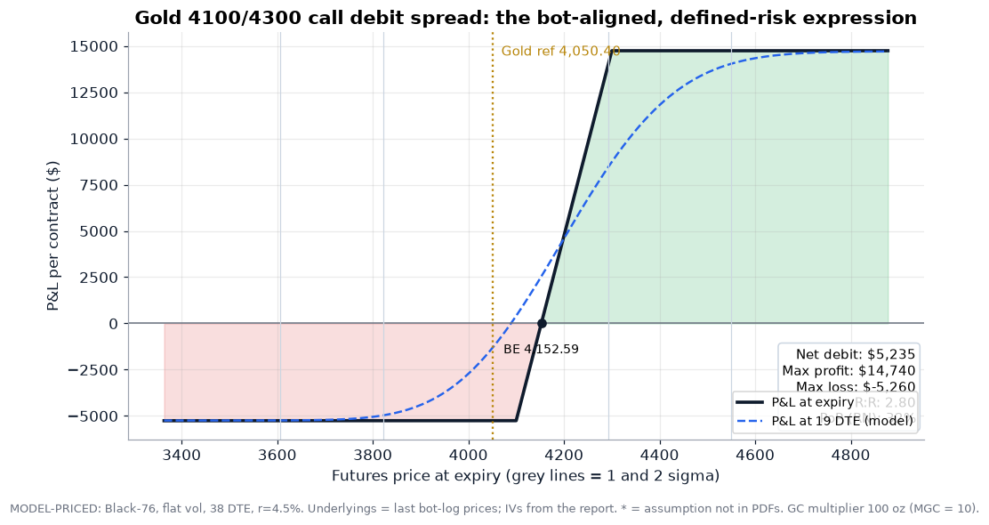
Structure: buy the 4100 call, sell the 4300 call (December, 38 DTE).
Cost: $5,235 per GC contract, or about $524 on MGC.
Profit and loss: maximum gain $14,740, maximum loss $5,260 (the debit plus financing).
Reward-to-risk: 2.80.
Breakeven: 4,152.59, which is +0.43σ.
Risk-neutral probability of profit: 32%.
This is the cleanest expression of the gold bot’s thesis. It uses the “0.30-0.50 delta, defined-risk call spread” structure the options PDF recommends for a long bot. It caps the loss at the debit, so the bot’s 91.6%-of-capital drawdown problem goes away. And because the short 4300 call sells back some of the 18% IV, the net vega is modest (see the Greeks below). The cost is the cap: gold above 4,300 earns nothing extra. Given the bot’s history of one or two monster months, that cap is a real trade-off, which is why the next structure exists.
4.2 Tier A #2: the zero-cost gold spread collar
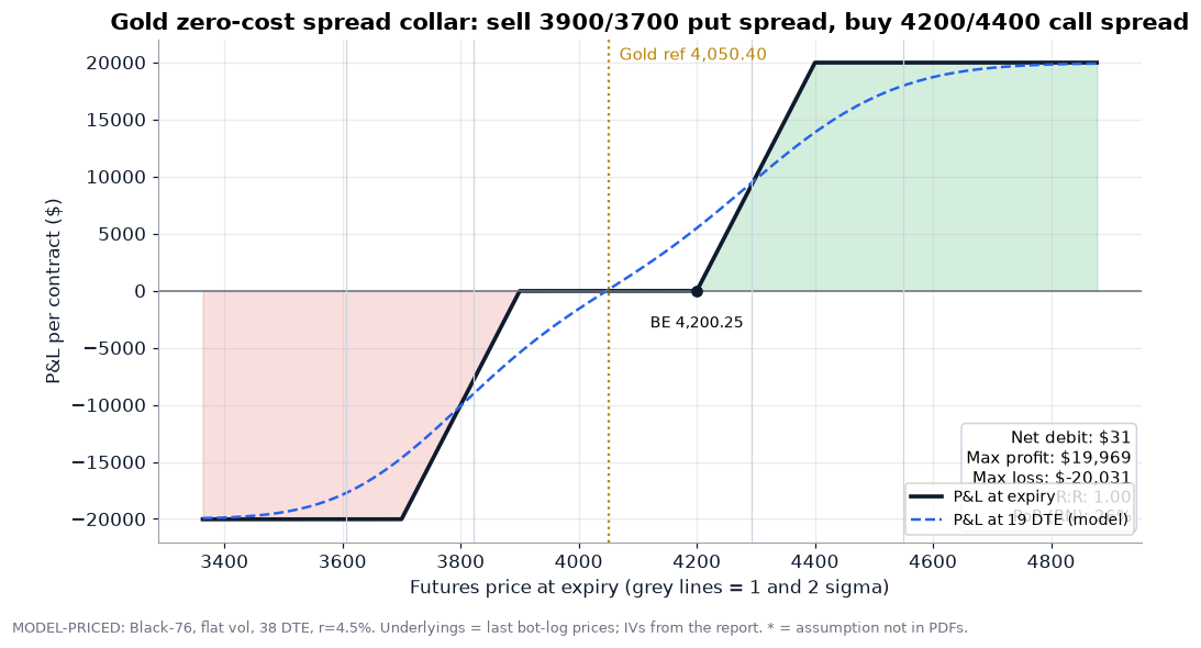
Structure: sell the 3900/3700 put spread and buy the 4200/4400 call spread.
Net cost: about $31, effectively zero.
Profit and loss: maximum gain $19,969 above 4,400, maximum loss $20,031 below 3,700.
Flat zone: about $0 between 3,900 and 4,200.
Probabilities (risk-neutral): 26% of finishing above the 4,200 breakeven. Only 14% of losing at least half the maximum loss.
The report describes the institutional version: “sold GCZ6 1,800 puts to finance 1,900/2,000 call spreads (yield enhancement trade)”. I mapped it by moneyness and added a long 3700 put to define the downside. Reward-to-risk is exactly 1.0, as you’d expect for a symmetric zero-cost structure under flat vol. The edge has to come from your directional view and from skew. In a gold market where safe-haven demand bids calls, the 25-delta risk reversal is often positive, which would make this structure even cheaper to put on. It’s the best structure if you share the bot’s long-gold conviction and want a full 4,400 upside without paying premium. You accept a hard −$20k tail per GC contract, so on micros it’s −$2k.
4.3 Tier A #3: ZN 108/106 put debit spread
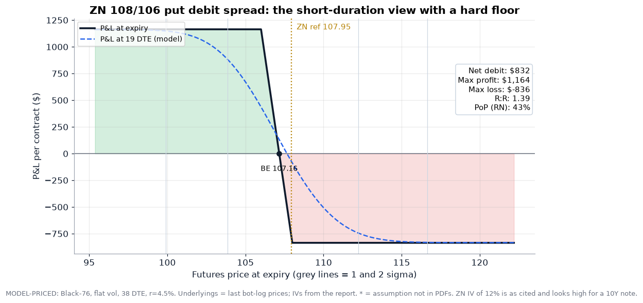
Structure: buy the 108 put, sell the 106 put.
Cost: $832.
Profit and loss: maximum gain $1,164, maximum loss $836.
Reward-to-risk: 1.39.
Breakeven: 107.16, which is ‑0.19σ.
Risk-neutral probability of profit: 43%.
This replaces the ZN bot’s 36x-levered outright short with a hard floor. The October drawdown of four straight stops ($14,966 on five contracts) would have cost at most $836 per spread. You give up the outsized August-September runs. The ZN IV of 12% is taken from the report and looks rich for a 10-year note. If true vol is lower, this spread is cheaper than shown, and its reward-to-risk improves.
4.4 Avoid: short ZN with the report’s 110/115 call-spread hedge
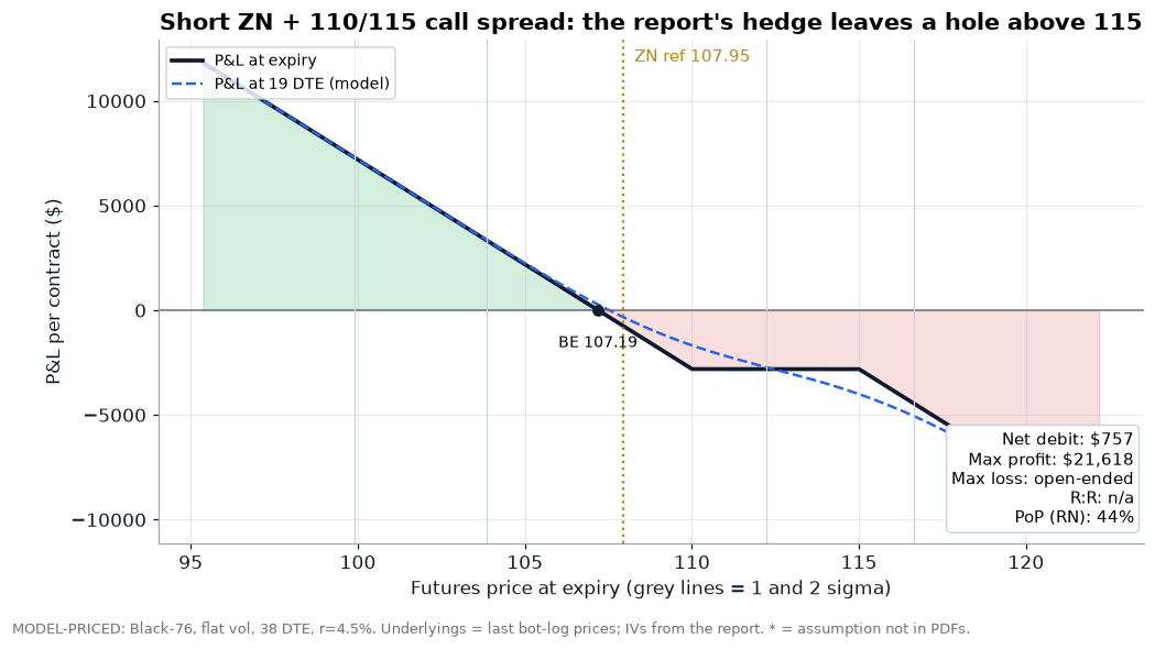
The report’s “directional” rates idea is: short ZN futures and hedge the upside with a long 110 call / short 115 call. The payoff diagram shows the flaw. The hedge stops working above 115. Short futures plus a call spread equals a capped hedge on an uncapped liability. In a duration squeeze (a soft CPI on a crowded 450K-contract short), price runs through 115 and the loss becomes open-ended again. If you want the short-futures leg, hedge it with a long call (a synthetic put) or just own the put spread above. Lesson: always plot the payoff of the whole package, not the hedge in isolation.
4.5 Tier B: hedges and report-only views
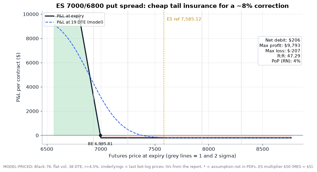
ES 7000/6800 put spread. This costs $206 per ES contract. It pays up to $9,793 if ES finishes below 6,800, a reward-to-risk of 47 to 1, with a risk-neutral probability of profit of only 4%. It’s the report’s “10% correction hedge”, priced at 14% flat vol. In a real market the downside skew would make the 7000 put richer than this. Even so, at about 0.05% of an ES contract’s $379k notional, it’s cheap insurance against the scenario the macro section worries about: hot CPI, a December hike and a yield-led equity selloff, given the report’s ES vs 10-year note correlation of ‑0.85.
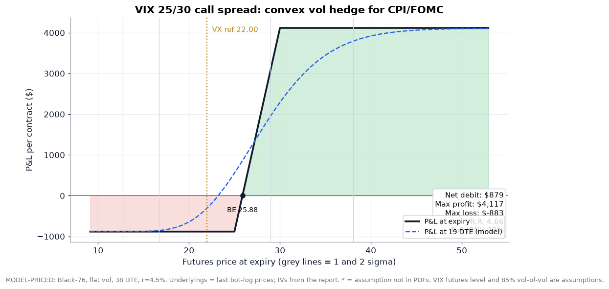
VIX 25/30 call spread. This costs $879 and pays up to $4,117 (4.7 to 1), with a breakeven at 25.88. The VIX futures level (22) and the 85% vol-of-vol are my assumptions. The PDFs give conflicting VIX readings and no VIX vol. The report says institutions bought exactly this spread to hedge the December FOMC. It’s convex, it’s defined risk, and it pays most in the scenario where the long-gold position might also be hurting (a dash for USD cash).
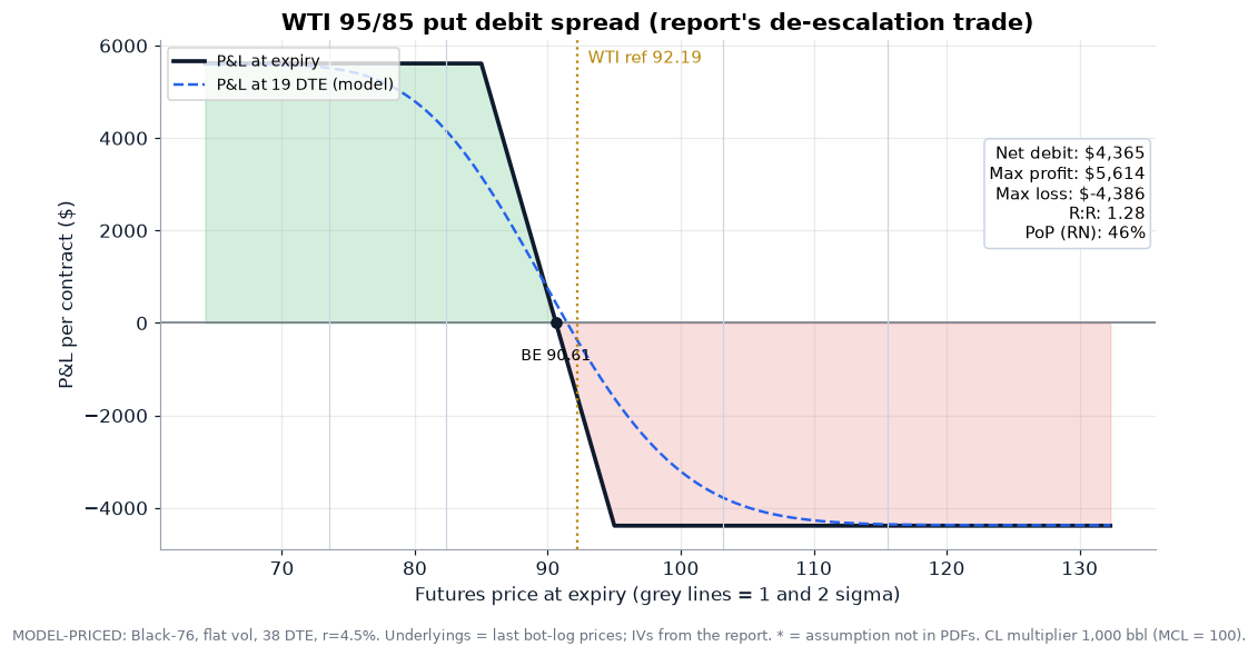
WTI 95/85 put spread. This costs $4,365 and pays up to $5,614 (1.28 to 1), with a breakeven at 90.61 and a 46% probability of profit. The report’s “de-escalation” trade has a coherent driver (a Hormuz deal and OPEC+ recovery), but no bot evidence: the crude momentum bot lost trading both directions. Because the 95 strike is in the money from 92.19, this behaves like a capped short-crude position, so you’re mostly paying intrinsic value. It’s a reasonable spread for a discretionary view, but nothing more.
4.6 Tier C: speculative
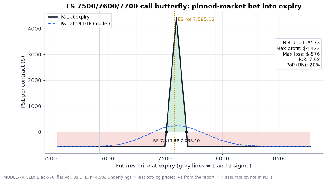
ES 7500/7600/7700 call butterfly. This costs $573 and pays up to $4,422 at a 7,600 pin (7.7 to 1), with breakevens at 7,511 and 7,688 and a 20% probability of profit. It’s a “pinned market into expiry” bet. That’s the opposite of what CPI plus FOMC implies, but it’s a cheap way to sell the elevated vol with defined risk.
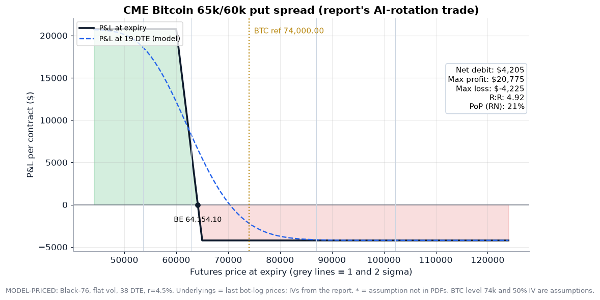
CME Bitcoin 65k/60k put spread. This costs $4,205 (per 5-BTC contract) and pays up to $20,775 (4.9 to 1), with a breakeven at 64,154. Both the BTC level and its vol are assumptions. The PDFs only say BTC is “below its 50-week MA ($75K)”. The thesis (”AI selloff rotation”, “quantum landmines”) is narrative only.
4.7 Avoid: the NatGas short strangle
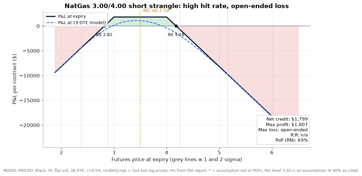
NatGas 3.00/4.00 short strangle. This collects $1,799 per 10,000 MMBtu contract, with a 69% risk-neutral probability of profit and breakevens at 2.82 and 4.18. The loss is open-ended in both directions. The report likes it because NG IV is 60%+ after an 8% short squeeze. That is precisely when the tails are fattest: winter weather, the TTF crisis the report itself describes, and LNG at $30+. A 69% hit rate with unlimited losses is how short-vol books blow up. If you must sell NG vol, sell a defined-risk iron condor.
4.8 The Greeks of the top structure
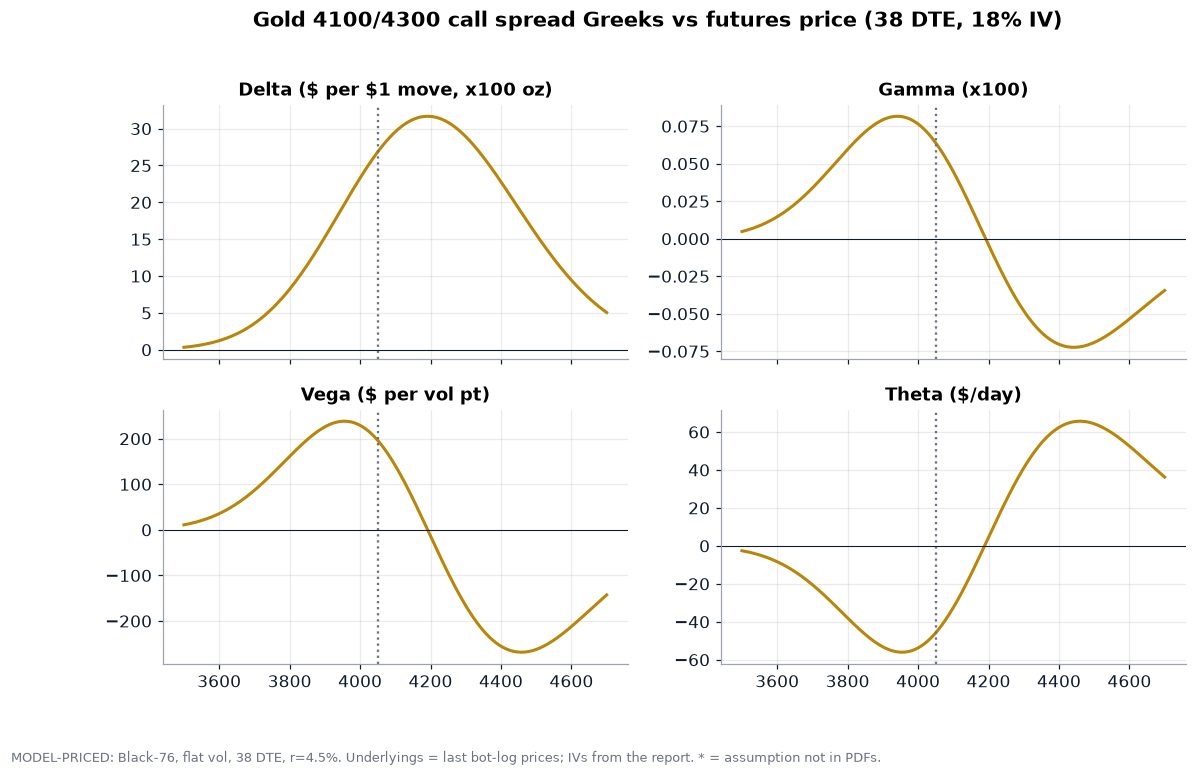
The 4100/4300 call spread is a delta trade with controlled second-order risk:
Delta peaks around the 4,200 midpoint at about +$32 per $1 move per GC contract, roughly a third of a future. At today’s 4,050 it’s about +$27.
Gamma flips sign across the 4,200 midpoint.
Vega is long below about 4,190 and short above it. At today’s price it’s about +$196 per vol point, and it’s close to zero at the centre, so a post-CPI vol crush costs little once the trade is working.
Theta works against you when the spread is out of the money, and for you once gold is above the short strike.
This is the profile the options PDF describes for swing trades: enough delta to express the view, without paying for vega you don’t need.
4.9 Futures and spread strategies
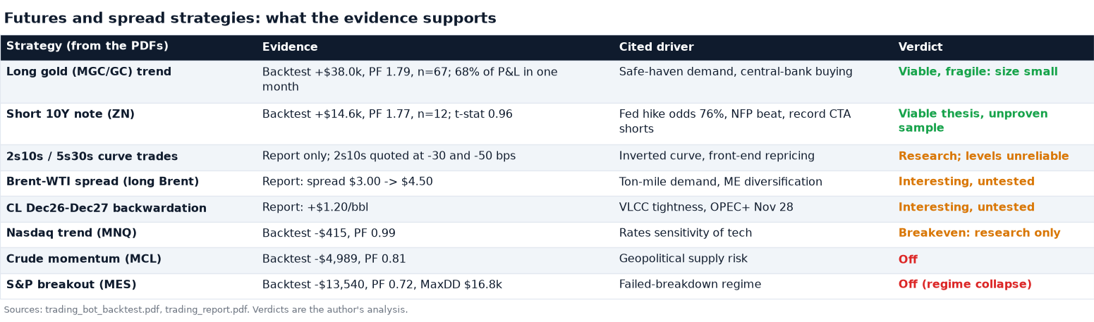
On the futures side, the evidence ranks the same way. Long gold and short ZN have backtests behind them. Curve trades, the Brent-WTI spread and the CL backwardation trade have plausible drivers in the report but no tested system. The three momentum bots on equity indices and crude are off. The two spread ideas (Brent over WTI, CLZ6-CLZ7 backwardation) are the most interesting untested strategies. They’re driven by the freight shock, a structural factor that a four-hour momentum signal won’t see.
5. Sizing: Kelly, drawdown and the regime switch
5.1 Growth-optimal sizing for a binary-payoff bot
If a bot wins b units per unit risked with probability p, and you risk a fraction f of equity on each trade, the expected log-growth per trade and the growth-optimal (Kelly) fraction are:
g(f) = p * ln(1 + f*b) + (1 - p) * ln(1 - f)
f*   = p - (1 - p) / b
For the gold bot (p = 0.507, b = 1.737), f* = 22.3%, which matches the PDF’s 22.4% Kelly figure. For ZN, f* = 21.7%. MNQ, MCL and MES have negative Kelly fractions, which is the mathematically polite way of saying “don’t trade this”.
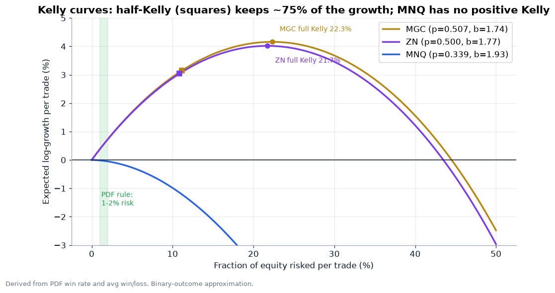
The curve is flat near the top. Half-Kelly keeps about 75% of the growth rate for a fraction of the variance. Betting more than about twice Kelly makes growth negative even with a positive edge.
5.2 What Kelly does to drawdowns
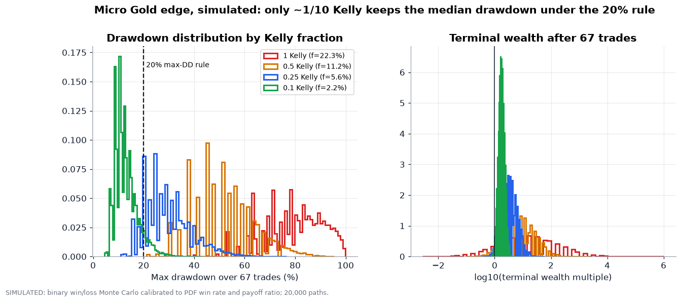
I simulated 20,000 paths of 67 gold-bot trades, using its win rate and payoff ratio. Medians across paths:

Those multiples are simulated and assume the backtest edge persists exactly, which Section 3.7 says is roughly a coin flip. The drawdown column is the useful one. Only around one-tenth Kelly (about 2% risk per trade) keeps the median drawdown under the 20% rule, and even then about 8% of paths (roughly 1 in 12) breach it. The PDF’s “never risk more than 1-2% per trade” rule sits right there. It’s the one rule in the 407-rule database the numbers fully back up.
A practical refinement is to shrink Kelly for estimation error. If the edge estimate has standard error se, a common approach is:
f_shrunk = f* × max(0, 1 − (z × se / edge)) with z ≈ 1 for a one-sigma haircut
For gold, with t ≈ 2.32, that’s roughly f* × (1 − 1/2.32), about 0.57 × f*, before any deflation for multiple testing. With the deflated PSR near 60%, one-tenth Kelly isn’t conservative. It’s about right.
5.3 The vol-regime switch, and why it needs one data feed
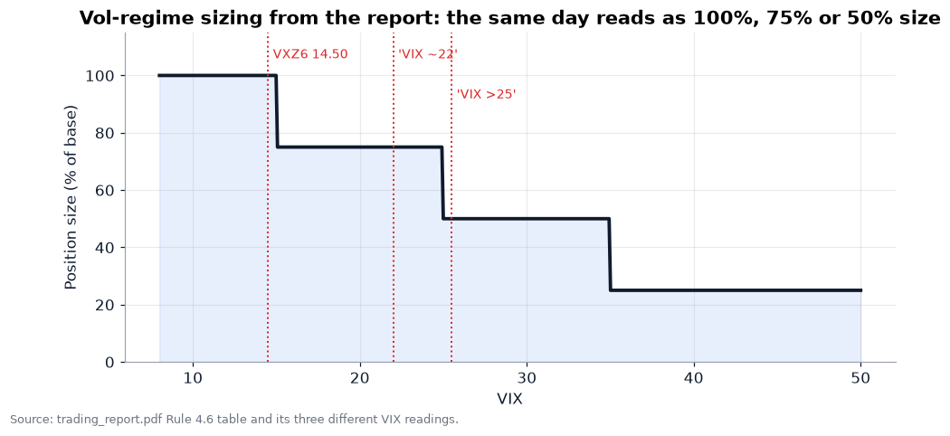
The report’s regime rule cuts size by 25% between VIX 15 and 25, by 50% between 25 and 35, and by 75% above 35. It’s sensible and widely used, but in this run the same document gives VIX readings of 14.50 (VXZ6), “~22” and “>25”. Depending on which paragraph you read, that’s full size, three-quarters or half. In code, a step function like this should read one authoritative series, ideally VIX futures settlement rather than a narrative. It should also be smoothed or given hysteresis so a reading of 24.9 vs 25.1 doesn’t flip size every day:
regime_t = clip(regime_{t-1}, lower = bucket(VIX_t - h), upper = bucket(VIX_t + h)) // h ≈ 1 VIX pt
5.4 Putting it together: an illustrative allocation
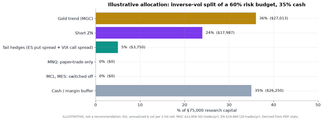
Here’s one illustrative way to allocate the $75,000 research book. Take a 60% risk budget and split it between the two surviving theses by inverse volatility, using annualised dollar vol per one-lot set (gold about $12,958, ZN about $19,460). That gives gold about 36% and ZN about 24%. Add 5% for the ES put-spread and VIX call-spread tail hedges and keep 35% in cash as a margin buffer. The PDF’s own leverage rules (”use only 30-50% of available margin”, “maintain 2-3x maintenance margin”) point to the same place. MNQ stays in paper trading and MCL and MES are switched off. The weights are a worked example of the method, not a recommendation.
Because gold and real yields are cited at about ‑0.75 correlation, the gold-long and ZN-short sleeves partly offset in a pure real-yield shock. The scenario that hurts both is a growth scare where yields fall (ZN rallies) and gold sells off in a dash for USD cash. That’s exactly the scenario the VIX call spread and the ES put spread are there to pay in.
6. The quant toolkit: equations you can copy
Every equation below is plain text, so it pastes cleanly into code, a notebook or a LaTeX editor. LaTeX versions of the core formulas are at the end of the section.
6.1 Options on futures (Black-76)
d1 = [ ln(F/K) + 0.5*σ²*T ] / (σ*√T)          d2 = d1 − σ*√T          DF = e^(−r*T)

Call  C = DF * [ F*N(d1) − K*N(d2) ]
Put   P = DF * [ K*N(−d2) − F*N(−d1) ]
Parity  C − P = DF * (F − K)

Delta_call = DF*N(d1)          Delta_put = −DF*N(−d1)
Gamma      = DF*φ(d1) / (F*σ*√T)
Vega       = DF*F*φ(d1)*√T                   (per 1.00 of vol; ÷100 per vol point)
Theta_call = −DF*F*φ(d1)*σ/(2√T) + r*C        (per year; ÷365 per day)
Vanna      = −DF*φ(d1)*d2/σ                   Volga = Vega*d1*d2/σ

1-sigma move to expiry  = F*σ*√T     ;   1-day move ≈ F*σ/√252
Risk-neutral P(F_T > X) = N( [ln(F/X) − 0.5σ²T] / (σ√T) )
For vertical spreads with width W = K2 − K1 and net debit D, the payoff numbers follow directly:
Call debit spread:  max loss = D,  max gain = W − D,  breakeven = K1 + D,  R:R = (W − D)/D
Put  debit spread:  max loss = D,  max gain = W − D,  breakeven = K2 − D
Butterfly K1<K2<K3: max gain = (K2 − K1) − D at F_T = K2;  breakevens K1 + D and K3 − D
For example, the ZN 108/106 put spread has W = 2.00 points × $1,000 = $2,000 and D = $832, so the maximum gain is $1,168 before financing ($1,164 after). That matches the engine’s output.
6.2 Volatility, skew and the vol risk premium
EWMA variance:      σ²_t = λ*σ²_{t−1} + (1−λ)*r²_{t−1}          λ ≈ 0.94 (daily)
Vol-of-vol:         VoV = stdev( Δ ln σ_implied ) * √252
Variance risk prem: VRP = σ²_implied − σ²_realised             (> 0 ⇒ options rich)
SVI smile:          w(k) = a + b*[ ρ*(k − m) + √((k − m)² + s²) ],   k = ln(K/F), σ(k) = √(w/T)
25Δ risk reversal:  RR25 = σ(25Δ call) − σ(25Δ put)            (< 0 ⇒ put skew)
25Δ butterfly:      BF25 = ½[σ(25Δ call) + σ(25Δ put)] − σ_ATM  (> 0 ⇒ fat tails priced)
Skew-adjusted delta: Δ_adj = Δ_BS + Vega * ∂σ/∂F
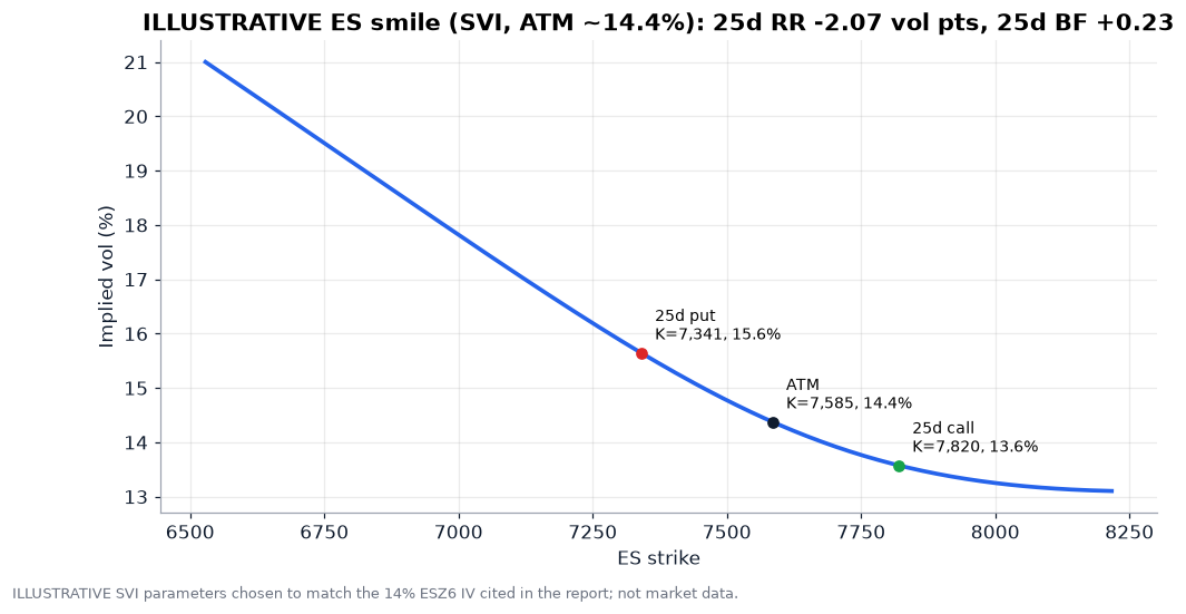
The smile above is illustrative. I picked SVI parameters to match the 14% ESZ6 IV the report cites, which gives a 25-delta risk reversal of ‑2.07 vol points and a butterfly of +0.23. The chain PDF returned no live strikes, so there’s nothing real to fit in this run. With live data, RR25 and BF25 are the two numbers to track daily. A deepening negative RR25 into CPI means institutions are paying up for exactly the put spreads in Section 4.5, which makes them more expensive than my flat-vol prices suggest.
6.3 Performance and tail metrics
Expectancy       E   = p*W̄ − (1 − p)*L̄
Profit factor    PF  = Σ wins / |Σ losses|  = p*W̄ / ((1 − p)*L̄)
Payoff ratio     b   = W̄ / L̄               Breakeven win rate p* = 1/(1 + b)
Sharpe           SR  = mean(r) / stdev(r) * √(periods per year)
Sortino          SoR = mean(r) / downside_dev(r) * √(ppy),   downside_dev = √(mean(min(r,0)²))
Calmar           CR  = annual return / max drawdown
Max drawdown     MDD = max_t (peak_t − equity_t) / peak_t         ← denominator = PEAK equity
VaR_α            = −quantile_{1−α}(r)        CVaR_α = −E[ r | r ≤ quantile_{1−α}(r) ]
SQN              = √n * mean(trade) / stdev(trade)
6.4 Is the Sharpe real? PSR and the deflated Sharpe
PSR(SR*) = N( (SR − SR*) * √(n − 1) / √(1 − γ3*SR + ((γ4 − 1)/4)*SR²) )
    γ3 = skewness, γ4 = kurtosis (3 for normal), SR per period, n = observations

E[max SR | N skill-less trials] ≈ √V[SR] * [ (1 − γ)*Z⁻¹(1 − 1/N) + γ*Z⁻¹(1 − 1/(N*e)) ]
    γ = 0.5772 (Euler–Mascheroni), Z⁻¹ = inverse normal CDF

Deflated Sharpe = PSR evaluated at SR* = E[max SR]
That’s the calculation that took gold from 98.8% to 60.2% in Section 3.7.
6.5 Sizing
Kelly (binary)       f* = p − (1 − p)/b
Kelly (continuous)   f* = μ / σ²                     (μ, σ of the strategy's excess return)
Fixed-fractional     contracts = floor( equity * risk% / (stop_distance * multiplier) )
Vol targeting        contracts = floor( target_$vol / (σ_daily * F * multiplier * √h) )
Inverse-vol weights  w_i = (1/σ_i) / Σ_j (1/σ_j)
DV01 curve hedge     n_short / n_long = DV01_long / DV01_short    (duration-neutral steepener)
The fixed-fractional line is the PDF’s own position-size rule, written as a formula. It’s generic risk management, not a bot rule.
6.6 Microstructure for execution
Top-of-book imbalance   I = (Q_bid − Q_ask) / (Q_bid + Q_ask)          ∈ [−1, 1]
Microprice              P_micro = P_ask * Q_bid/(Q_bid+Q_ask) + P_bid * Q_ask/(Q_bid+Q_ask)
Order-flow imbalance    e_n = 1{Pb_n ≥ Pb_{n−1}}*qb_n − 1{Pb_n ≤ Pb_{n−1}}*qb_{n−1}
                            − 1{Pa_n ≤ Pa_{n−1}}*qa_n + 1{Pa_n ≥ Pa_{n−1}}*qa_{n−1}
                        OFI_k = Σ_{n in window k} e_n ;   ΔP_k ≈ β * OFI_k / depth
Square-root impact      cost/price ≈ Y * σ_daily * √(Q / ADV),   Y ≈ 0.5–1
Almgren–Chriss          x_j = X * sinh(κ(T − t_j)) / sinh(κT),
                        cosh(κτ) = 1 + λσ²τ²/(2η̃)
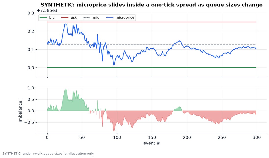
The microprice is a better short-horizon fair value than the mid. With 180 lots bid and 60 offered on a 7,585.00/7,585.25 MES quote, imbalance is +0.5 and the microprice is 7,585.1875, three-quarters of the way to the offer. That tells you the offer is likely to be lifted, so passive bids are unlikely to fill. The chart uses synthetic queue sizes.
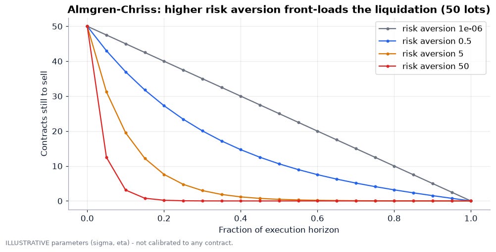
Almgren-Chriss formalizes the trade-off between impact and risk. A risk-neutral trader liquidates in a straight line (TWAP). A risk-averse one front-loads to cut exposure to price moves. For a micro-futures bot trading a few lots, impact is negligible. For anyone scaling the same signal to hundreds of standard contracts around CPI, this schedule matters more than the entry signal.
6.7 Carry, basis and spreads
Cost of carry           F = S * e^{(r − y)T}           (y = convenience yield / dividend yield)
Annualised roll yield   RY = ln(F_near / F_far) / (T_far − T_near)       (> 0 in backwardation)
Spread z-score          z_t = (s_t − mean_N(s)) / stdev_N(s),  s = Brent − WTI
Crack spread (3-2-1)    = (2*RB*42 + 1*HO*42 − 3*CL) / 3     ($/bbl; RB, HO quoted in $/gal)
The report cites a CLZ6-CLZ7 spread of +$1.20 at about $92 WTI. Over one year that’s an annualised roll yield of about ln(92.19/90.99), roughly +1.3% for a long-front holder. It’s modest, but it’s positive carry on the same side as the freight-driven tightness story. The calculation uses the trade-log price and the spread the report cites.
6.8 LaTeX versions (core formulas)
d_{1}=\frac{\ln(F/K)+\tfrac12\sigma^{2}T}{\sigma\sqrt{T}},\quad d_{2}=d_{1}-\sigma\sqrt{T}
C=e^{-rT}\left[F\,N(d_{1})-K\,N(d_{2})\right],\quad P=e^{-rT}\left[K\,N(-d_{2})-F\,N(-d_{1})\right]
\Gamma=\frac{e^{-rT}\varphi(d_{1})}{F\sigma\sqrt{T}},\qquad \mathcal{V}=e^{-rT}F\varphi(d_{1})\sqrt{T}
g(f)=p\ln(1+fb)+(1-p)\ln(1-f),\qquad f^{*}=p-\frac{1-p}{b}
\widehat{PSR}(SR^{*})=\Phi\!\left(\frac{(\widehat{SR}-SR^{*})\sqrt{n-1}}{\sqrt{1-\hat\gamma_{3}\widehat{SR}+\frac{\hat\gamma_{4}-1}{4}\widehat{SR}^{2}}}\right)
P_{\text{micro}}=P_{a}\frac{Q_{b}}{Q_{b}+Q_{a}}+P_{b}\frac{Q_{a}}{Q_{b}+Q_{a}},\qquad x_{j}=X\frac{\sinh\kappa(T-t_{j})}{\sinh\kappa T}
7. Python you can run
Each block below ran cleanly on Python 3 with numpy and scipy. The outputs shown are the actual outputs. Save the first block as black76.py. The second imports it.
7.1 Black-76, Greeks, implied vol and a multi-leg payoff engine
# black76.py -- Black-76 pricing, Greeks, implied vol and a multi-leg payoff engine
# for options on futures. Pure numpy/scipy; save as black76.py to reuse below.
import numpy as np
from scipy.stats import norm
from scipy.optimize import brentq

def b76(F, K, T, sigma, r=0.045, kind="C"):
    """Black-76 price of a European option on a futures contract."""
    sq = sigma * np.sqrt(T)
    d1 = (np.log(F / K) + 0.5 * sq * sq) / sq
    d2 = d1 - sq
    df = np.exp(-r * T)
    if kind == "C":
        return df * (F * norm.cdf(d1) - K * norm.cdf(d2))
    return df * (K * norm.cdf(-d2) - F * norm.cdf(-d1))

def b76_greeks(F, K, T, sigma, r=0.045, kind="C"):
    sq = sigma * np.sqrt(T)
    d1 = (np.log(F / K) + 0.5 * sq * sq) / sq
    d2 = d1 - sq
    df = np.exp(-r * T)
    pdf = norm.pdf(d1)
    price = b76(F, K, T, sigma, r, kind)
    delta = df * norm.cdf(d1) if kind == "C" else -df * norm.cdf(-d1)
    gamma = df * pdf / (F * sq)
    vega = df * F * pdf * np.sqrt(T)            # per 1.00 vol (divide by 100 for 1 vol pt)
    theta = -df * F * pdf * sigma / (2 * np.sqrt(T)) + r * price   # per year
    vanna = -df * pdf * d2 / sigma               # d(delta)/d(sigma)
    volga = vega * d1 * d2 / sigma               # d(vega)/d(sigma)
    return dict(price=price, delta=delta, gamma=gamma, vega=vega, theta=theta,
                vanna=vanna, volga=volga)

def implied_vol(price, F, K, T, r=0.045, kind="C"):
    f = lambda s: b76(F, K, T, s, r, kind) - price
    return brentq(f, 1e-4, 5.0, xtol=1e-10)

def evaluate(legs, F, T, sigma, r=0.045, mult=1.0, n=40001):
    """legs: list of (kind, strike, qty) with kind in {'C','P','F'}; qty>0 = long.
    Returns net premium, max profit/loss, breakevens and risk-neutral P(profit) at expiry."""
    prem = 0.0
    for kind, K, q in legs:
        if kind != "F":
            prem += q * b76(F, K, T, sigma, r, kind)
    sd = sigma * np.sqrt(T)
    x = F * np.exp(np.linspace(-6 * sd, 6 * sd, n))      # +-6 sigma terminal grid
    pay = np.zeros_like(x)
    for kind, K, q in legs:
        if kind == "C":
            pay += q * np.maximum(x - K, 0)
        elif kind == "P":
            pay += q * np.maximum(K - x, 0)
        else:                                       # futures leg entered at K
            pay += q * (x - K)
    pnl = (pay - prem * np.exp(r * T)) * mult        # premium financed to expiry
    # does the P&L keep falling (or rising) at the edges of a +-6 sigma grid?
    tol = 1e-9 * max(1.0, abs(mult))
    open_loss = bool(pnl[0] < pnl[1] - tol or pnl[-1] < pnl[-2] - tol)
    open_gain = bool(pnl[0] > pnl[1] + tol or pnl[-1] > pnl[-2] + tol)
    s = np.sign(pnl)
    be = x[np.where(np.diff(s) != 0)[0]]
    # lognormal terminal density of F_T under the pricing measure (driftless)
    z = np.log(x / F) / sd + 0.5 * sd
    w = norm.pdf(z) * np.gradient(z)
    pop = float(np.sum(w[pnl > 0]) / np.sum(w))        # P(profit)
    p_loss = float(np.sum(w[pnl <= 0.5 * pnl.min()]) / np.sum(w))  # P(lose >= half of max loss)
    ev = float(np.sum(w * pnl) / np.sum(w))            # risk-neutral EV (should be ~0)
    return dict(premium=prem * mult, max_profit=pnl.max(), max_loss=pnl.min(),
                rr=pnl.max() / abs(pnl.min()) if pnl.min() < 0 else np.inf,
                breakevens=be, pop=pop, p_loss=p_loss, ev=ev, x=x, pnl=pnl,
                open_loss=open_loss, open_gain=open_gain)

if __name__ == "__main__":
    T = 38 / 365            # 38 DTE: the Dec-18-2026 expiry quoted in the chain PDF
    F, iv = 4050.40, 0.18   # last gold price in the bot log; GCZ6 IV cited in the report
    g = b76_greeks(F, 4000, T, iv, kind="C")
    print({k: round(float(v), 4) for k, v in g.items()})
    print("round-trip IV:", round(implied_vol(g["price"], F, 4000, T), 6))
Output:
{'price': 120.0456, 'delta': 0.5938, 'gamma': 0.0016, 'vega': 503.6441, 'theta': -429.985, 'vanna': -0.3994, 'volga': 127.6912}
round-trip IV: 0.18
7.2 Price and rank the report’s structures
# rank_structures.py -- price and rank the options-on-futures structures named in the
# 2026-11-09 report with Black-76. Flat vol per underlying (no skew) => model prices.
import numpy as np
from black76 import evaluate

T = 38 / 365
R = 0.045   # "~4.50%" SOFR pricing cited in the report
# name, underlying F, vol, contract multiplier, legs (kind, strike, qty)
BOOK = [
 ("Gold zero-cost: sell 3900/3700 PS, buy 4200/4400 CS", 4050.40, 0.18, 100,
    [("P", 3700, +1), ("P", 3900, -1), ("C", 4200, +1), ("C", 4400, -1)]),
 ("Gold 4100/4300 call debit spread",              4050.40, 0.18, 100,
    [("C", 4100, +1), ("C", 4300, -1)]),
 ("ZN 108/106 put debit spread",                    107.95, 0.12, 1000,
    [("P", 108, +1), ("P", 106, -1)]),
 ("Short ZN + 110/115 call spread (report hedge)",  107.95, 0.12, 1000,
    [("F", 107.95, -1), ("C", 110, +1), ("C", 115, -1)]),
 ("WTI 95/85 put debit spread",                       92.19, 0.35, 1000,
    [("P", 95, +1), ("P", 85, -1)]),
 ("ES 7000/6800 put spread (tail hedge)",           7585.12, 0.14, 50,
    [("P", 7000, +1), ("P", 6800, -1)]),
 ("ES 7500/7600/7700 call butterfly",               7585.12, 0.14, 50,
    [("C", 7500, +1), ("C", 7600, -2), ("C", 7700, +1)]),
 ("VIX 25/30 call spread (F=22, vol 85%*)",           22.00, 0.85, 1000,
    [("C", 25, +1), ("C", 30, -1)]),
 ("BTC 65k/60k put spread (F=74k*, vol 50%*)",      74000.0, 0.50, 5,
    [("P", 65000, +1), ("P", 60000, -1)]),
 ("NatGas 3.00/4.00 short strangle (F=3.50*)",         3.50, 0.60, 10000,
    [("P", 3.00, -1), ("C", 4.00, -1)]),
]

def rank(book=BOOK):
    rows = []
    for name, F, vol, mult, legs in book:
        e = evaluate(legs, F, T, vol, R, mult)
        sd = vol * np.sqrt(T)
        be_sig = [float(np.log(b / F) / sd) for b in e["breakevens"]]
        rows.append(dict(name=name, F=F, vol=vol, premium=e["premium"],
                         max_profit=e["max_profit"], max_loss=e["max_loss"],
                         rr=e["rr"], pop=e["pop"], p_loss=e["p_loss"], ev=e["ev"], be=e["breakevens"], be_sigma=be_sig,
                         open_loss=e["open_loss"], open_gain=e["open_gain"],
                         x=e["x"], pnl=e["pnl"]))
    # payoff-efficiency score: reward:risk scaled by the risk-neutral hit rate,
    # penalised hard for open-ended loss. ~1.0 means "fairly priced lottery".
    for r in rows:
        r["score"] = 0.0 if r["open_loss"] else r["rr"] * r["pop"] / (1 - r["pop"])
    return rows

if __name__ == "__main__":
    for r in rank():
        be = ", ".join(f"{b:,.2f} ({s:+.2f}sd)" for b, s in zip(r["be"], r["be_sigma"]))
        print(f'{r["name"][:46]:46s} prem {r["premium"]:>10,.0f}  maxP {r["max_profit"]:>10,.0f} '
              f'maxL {r["max_loss"]:>10,.0f}  RR {r["rr"]:5.2f}  PoP {r["pop"]:5.1%}  P(>=half maxL) {r["p_loss"]:5.1%}  EV {r["ev"]:6.0f}  '
              f'openLoss {r["open_loss"]!s:5s}  BE {be}')
Output:
Gold zero-cost: sell 3900/3700 PS, buy 4200/44 prem         31  maxP     19,969 maxL    -20,031  RR  1.00  PoP 25.6%  P(>=half maxL) 14.3%  EV     -0  openLoss False  BE 4,200.25 (+0.63sd)
Gold 4100/4300 call debit spread               prem      5,235  maxP     14,740 maxL     -5,260  RR  2.80  PoP 32.3%  P(>=half maxL) 63.6%  EV      0  openLoss False  BE 4,152.59 (+0.43sd)
ZN 108/106 put debit spread                    prem        832  maxP      1,164 maxL       -836  RR  1.39  PoP 43.3%  P(>=half maxL) 52.7%  EV     -0  openLoss False  BE 107.16 (-0.19sd)
Short ZN + 110/115 call spread (report hedge)  prem        757  maxP     21,618 maxL    -23,991  RR  0.90  PoP 43.5%  P(>=half maxL)  0.0%  EV      0  openLoss True   BE 107.19 (-0.18sd)
WTI 95/85 put debit spread                     prem      4,365  maxP      5,614 maxL     -4,386  RR  1.28  PoP 46.2%  P(>=half maxL) 45.4%  EV     -0  openLoss False  BE 90.61 (-0.15sd)
ES 7000/6800 put spread (tail hedge)           prem        206  maxP      9,793 maxL       -207  RR 47.29  PoP  3.9%  P(>=half maxL) 96.1%  EV     -0  openLoss False  BE 6,995.81 (-1.79sd)
ES 7500/7600/7700 call butterfly               prem        573  maxP      4,422 maxL       -576  RR  7.68  PoP 20.3%  P(>=half maxL) 78.4%  EV     -0  openLoss False  BE 7,511.47 (-0.22sd), 7,688.40 (+0.30sd)
VIX 25/30 call spread (F=22, vol 85%*)         prem        879  maxP      4,117 maxL       -883  RR  4.66  PoP 23.3%  P(>=half maxL) 74.8%  EV      0  openLoss False  BE 25.88 (+0.59sd)
BTC 65k/60k put spread (F=74k*, vol 50%*)      prem      4,205  maxP     20,775 maxL     -4,225  RR  4.92  PoP 21.1%  P(>=half maxL) 77.7%  EV      0  openLoss False  BE 64,154.10 (-0.89sd)
NatGas 3.00/4.00 short strangle (F=3.50*)      prem     -1,799  maxP      1,807 maxL    -70,017  RR  0.03  PoP 69.1%  P(>=half maxL)  0.0%  EV      0  openLoss True   BE 2.82 (-1.12sd), 4.18 (+0.92sd)
7.3 Re-derive the bot statistics, PSR and deflated Sharpe
# bot_metrics.py -- re-derive and stress-test the backtest statistics printed in the PDFs.
import numpy as np
from scipy.stats import norm

def edge_stats(p, avg_win, avg_loss, n):
    """Binary-outcome approximation from win rate and average win/loss."""
    b = avg_win / abs(avg_loss)                       # payoff ratio
    exp_ = p * avg_win - (1 - p) * abs(avg_loss)      # expectancy per trade ($)
    be_wr = 1 / (1 + b)                               # breakeven win rate
    kelly = p - (1 - p) / b                           # full Kelly fraction of risk capital
    pf = p * avg_win / ((1 - p) * abs(avg_loss))      # implied profit factor
    sd = np.sqrt(p * avg_win**2 + (1 - p) * avg_loss**2 - exp_**2)
    sr_t = exp_ / sd                                  # per-trade Sharpe
    return dict(b=b, expectancy=exp_, be_wr=be_wr, kelly=kelly, pf=pf,
                sd=sd, sr_trade=sr_t, sqn=np.sqrt(n) * sr_t, t_stat=np.sqrt(n) * sr_t)

def psr(sr, n, skew=0.0, kurt=3.0, sr_bench=0.0):
    """Probabilistic Sharpe Ratio (Bailey & Lopez de Prado), per-period SR."""
    den = np.sqrt(1 - skew * sr + (kurt - 1) / 4 * sr**2)
    return norm.cdf((sr - sr_bench) * np.sqrt(n - 1) / den)

def expected_max_sr(n_trials, var_sr):
    """Expected max Sharpe of n_trials skill-less strategies (False Strategy Theorem)."""
    g = 0.5772156649
    return np.sqrt(var_sr) * ((1 - g) * norm.ppf(1 - 1 / n_trials)
                              + g * norm.ppf(1 - 1 / (n_trials * np.e)))

def drawdown(pnl, start_capital):
    eq = start_capital + np.cumsum(np.r_[0.0, pnl])
    peak = np.maximum.accumulate(eq)
    dd = eq - peak
    i = int(np.argmin(dd))
    return dict(max_dd=-dd[i], dd_vs_peak=-dd[i] / peak[i], dd_vs_start=-dd[i] / start_capital,
                equity=eq, peak=peak)

def cvar(x, a=0.95):
    q = np.quantile(x, 1 - a)
    return q, x[x <= q].mean()

if __name__ == "__main__":
    bots = {  # win rate, avg win, avg loss, trades  (from trading_bot_backtest.pdf)
        "MGC": (0.507, 2535.20, -1459.64, 67), "ZN": (0.500, 5598.96, -3164.06, 12),
        "MNQ": (0.339, 2311.06, -1197.97, 56), "MCL": (0.317, 1057.03, -607.67, 63),
        "MES": (0.286, 1416.61, -792.31, 84)}
    for k, (p, w, l, n) in bots.items():
        s = edge_stats(p, w, l, n)
        print(f"{k:4s} b={s['b']:.2f} E=${s['expectancy']:8.0f} BE-WR={s['be_wr']:.1%} "
              f"Kelly={s['kelly']:+.1%} PF={s['pf']:.2f} SR/trade={s['sr_trade']:+.3f} "
              f"t={s['t_stat']:+.2f} PSR={psr(s['sr_trade'], n):.1%}")
    zn = np.array([-2193.08, 4051.34, -1824.78, 3515.62, 5558.04, 6406.25, 8906.25,
                   5156.25, -3532.37, -3867.19, -4068.08, -3498.88])
    d = drawdown(zn, 15000)
    print("ZN maxDD $%.2f = %.1f%% of peak equity, %.1f%% of start capital"
          % (d["max_dd"], 100 * d["dd_vs_peak"], 100 * d["dd_vs_start"]))
    print("ZN trade mean %.2f sd %.2f  SR/trade %.3f" % (zn.mean(), zn.std(ddof=1), zn.mean() / zn.std(ddof=1)))
    srs = np.array([edge_stats(*v)["sr_trade"] for v in bots.values()])
    e_max = expected_max_sr(len(srs), srs.var(ddof=1))
    print("cross-bot SR var %.4f  E[max SR | no skill, 5 trials] = %.3f" % (srs.var(ddof=1), e_max))
    s = edge_stats(*bots["MGC"])
    print("MGC deflated PSR vs E[max]: %.1f%%" % (100 * psr(s["sr_trade"], 67, sr_bench=e_max)))
Output:
MGC  b=1.74 E=$     566 BE-WR=36.5% Kelly=+22.3% PF=1.79 SR/trade=+0.283 t=+2.32 PSR=98.8%
ZN   b=1.77 E=$    1217 BE-WR=36.1% Kelly=+21.7% PF=1.77 SR/trade=+0.278 t=+0.96 PSR=81.7%
MNQ  b=1.93 E=$      -8 BE-WR=34.1% Kelly=-0.4% PF=0.99 SR/trade=-0.005 t=-0.04 PSR=48.5%
MCL  b=1.74 E=$     -80 BE-WR=36.5% Kelly=-7.6% PF=0.81 SR/trade=-0.103 t=-0.82 PSR=20.9%
MES  b=1.79 E=$    -161 BE-WR=35.9% Kelly=-11.3% PF=0.72 SR/trade=-0.161 t=-1.47 PSR=7.3%
ZN maxDD $14966.52 = 33.6% of peak equity, 99.8% of start capital
ZN trade mean 1217.45 sd 4797.64  SR/trade 0.254
cross-bot SR var 0.0442  E[max SR | no skill, 5 trials] = 0.251
MGC deflated PSR vs E[max]: 60.2%
7.4 Kelly growth and the fractional-Kelly Monte Carlo
# kelly_mc.py -- growth-optimal sizing and a Monte Carlo of fractional Kelly.
# SIMULATED: binary win/loss model calibrated to the PDF's win rate and payoff ratio.
import numpy as np

def growth(f, p, b):
    """Expected log growth per trade when risking fraction f (loss = f, win = f*b)."""
    f = np.asarray(f, dtype=float)
    return p * np.log1p(f * b) + (1 - p) * np.log1p(-f)

def simulate(p, b, f, n_trades, n_paths=20000, seed=7):
    rng = np.random.default_rng(seed)
    wins = rng.random((n_paths, n_trades)) < p
    r = np.where(wins, f * b, -f)
    eq = np.cumprod(1 + r, axis=1)
    peak = np.maximum.accumulate(np.c_[np.ones(n_paths), eq], axis=1)[:, 1:]
    mdd = (1 - eq / peak).max(axis=1)
    return eq[:, -1], mdd

if __name__ == "__main__":
    p, b = 0.507, 2535.20 / 1459.64           # Micro Gold bot (backtest PDF)
    k = p - (1 - p) / b
    print(f"full Kelly f* = {k:.3f}")
    for frac in (1.0, 0.5, 0.25, 0.10):
        f = frac * k
        tw, mdd = simulate(p, b, f, n_trades=67)
        print(f"{frac:>4.2f} Kelly: f={f:.3f}  g/trade={growth(f, p, b):.4f}  "
              f"median x{np.median(tw):6.2f}  P(loss)={np.mean(tw < 1):5.1%}  "
              f"median MDD={np.median(mdd):5.1%}  95th MDD={np.quantile(mdd, .95):5.1%}")
Output:
full Kelly f* = 0.223
1.00 Kelly: f=0.223  g/trade=0.0416  median x 16.52  P(loss)=13.8%  median MDD=81.6%  95th MDD=96.4%
0.50 Kelly: f=0.112  g/trade=0.0315  median x  8.32  P(loss)= 3.3%  median MDD=50.9%  95th MDD=74.5%
0.25 Kelly: f=0.056  g/trade=0.0186  median x  3.49  P(loss)= 1.9%  median MDD=29.1%  95th MDD=47.3%
0.10 Kelly: f=0.022  g/trade=0.0082  median x  1.73  P(loss)= 0.9%  median MDD=12.6%  95th MDD=21.9%
7.5 Vol tools: EWMA, vol-of-vol, VRP and 25-delta skew from an SVI smile
# volskew.py -- EWMA vol, vol-of-vol, variance risk premium and smile skew metrics.
import numpy as np
from scipy.stats import norm
from scipy.optimize import brentq

def ewma_vol(returns, lam=0.94, periods=252):
    v = np.empty_like(returns); v[0] = returns[:20].var()
    for i in range(1, len(returns)):
        v[i] = lam * v[i - 1] + (1 - lam) * returns[i - 1] ** 2
    return np.sqrt(v * periods)

def vol_of_vol(iv_series, periods=252):
    """Annualised std-dev of log changes in implied vol."""
    return np.std(np.diff(np.log(iv_series)), ddof=1) * np.sqrt(periods)

def vrp(implied, realised):
    """Variance risk premium in variance points (implied^2 - realised^2)."""
    return implied**2 - realised**2

def svi_total_var(k, a, b, rho, m, s):
    """Gatheral raw SVI: total implied variance w(k) at log-moneyness k."""
    return a + b * (rho * (k - m) + np.sqrt((k - m) ** 2 + s * s))

def strike_for_delta(F, T, target, kind, smile):
    """Solve for the log-moneyness whose Black-76 delta (undiscounted) equals target."""
    def f(k):
        vol = np.sqrt(smile(k) / T)
        d1 = (-k + 0.5 * vol * vol * T) / (vol * np.sqrt(T))
        return (norm.cdf(d1) if kind == "C" else norm.cdf(d1) - 1) - target
    return brentq(f, -2.0, 2.0)

def rr_bf_25d(F, T, smile):
    kc = strike_for_delta(F, T, 0.25, "C", smile)
    kp = strike_for_delta(F, T, -0.25, "P", smile)
    vc, vp, va = (np.sqrt(smile(k) / T) for k in (kc, kp, 0.0))
    return dict(rr25=vc - vp, bf25=0.5 * (vc + vp) - va, atm=va,
                k_call=F * np.exp(kc), k_put=F * np.exp(kp))

if __name__ == "__main__":
    T = 38 / 365
    # ILLUSTRATIVE equity-style smile with ATM ~14% (the ESZ6 IV cited in the report)
    smile = lambda k: svi_total_var(k, a=0.0011, b=0.012, rho=-0.70, m=0.01, s=0.08)
    print({k: round(float(v), 4) for k, v in rr_bf_25d(7585.12, T, smile).items()})
    print("VRP if IV=14%% and RV=11%%: %.4f var pts" % vrp(0.14, 0.11))
    rng = np.random.default_rng(1)
    r = rng.standard_t(4, 500) * 0.008
    print("EWMA vol (last):", round(float(ewma_vol(r)[-1]), 4))
    iv = 0.14 * np.exp(np.cumsum(rng.normal(0, 0.05, 250)))
    print("vol-of-vol:", round(float(vol_of_vol(iv)), 3))
Output:
{'rr25': -0.0207, 'bf25': 0.0023, 'atm': 0.1438, 'k_call': 7820.0675, 'k_put': 7340.5698}
VRP if IV=14% and RV=11%: 0.0075 var pts
EWMA vol (last): 0.1911
vol-of-vol: 0.805
7.6 Microstructure: imbalance, microprice, impact and Almgren-Chriss
# microstructure.py -- order-book imbalance, microprice, square-root impact and an
# Almgren-Chriss optimal liquidation schedule. Inputs below are ILLUSTRATIVE.
import numpy as np

def imbalance(bid_sz, ask_sz):
    return (bid_sz - ask_sz) / (bid_sz + ask_sz)

def microprice(bid, ask, bid_sz, ask_sz):
    """Size-weighted 'fair' price: leans toward the side about to be depleted."""
    I = bid_sz / (bid_sz + ask_sz)
    return ask * I + bid * (1 - I)

def multilevel_ofi(bids, asks, depth_decay=0.5):
    """Depth-weighted imbalance across L levels: weights w_l = decay**l."""
    w = depth_decay ** np.arange(len(bids))
    return float((w @ bids - w @ asks) / (w @ bids + w @ asks))

def sqrt_impact(q, adv, sigma_daily, y=0.7):
    """Square-root law: expected cost (fraction of price) of trading q vs ADV."""
    return y * sigma_daily * np.sqrt(q / adv)

def almgren_chriss(X, T, N, sigma, eta, lam):
    """Optimal holdings x_k for liquidating X over T in N steps (linear temp. impact eta,
    risk aversion lam, price vol sigma). kappa solves cosh(kappa*tau) = 1 + lam sigma^2 tau^2/(2 eta)."""
    tau = T / N
    kappa = np.arccosh(1 + lam * sigma**2 * tau**2 / (2 * eta)) / tau
    t = np.linspace(0, T, N + 1)
    return X * np.sinh(kappa * (T - t)) / np.sinh(kappa * T)

if __name__ == "__main__":
    bid, ask = 7585.00, 7585.25                 # one MES/ES tick wide (0.25)
    print("I =", imbalance(180, 60), " micro =", microprice(bid, ask, 180, 60))
    print("OFI(5 lvls) =", round(multilevel_ofi(np.array([180, 150, 120, 90, 80]),
                                                np.array([60, 140, 160, 130, 110])), 4))
    print(f"sqrt impact, 1% of ADV, 1.2% daily vol: {1e4 * sqrt_impact(0.01, 1, 0.012):.2f} bp")
    x = almgren_chriss(X=50, T=1.0, N=10, sigma=0.95, eta=0.05, lam=0.5)
    print("AC holdings:", np.round(x, 2))
Output:
I = 0.5  micro = 7585.1875
OFI(5 lvls) = 0.2187
sqrt impact, 1% of ADV, 1.2% daily vol: 8.40 bp
AC holdings: [50.   36.99 27.32 20.11 14.72 10.66  7.56  5.14  3.19  1.53  0.  ]
8. Ultra-low-latency C++ for the execution layer
None of the five bots needs nanoseconds. They trade four-hour bars. But the institutional structures above are traded against market makers who do, and the same infrastructure decides your fill quality around CPI prints. Here are four self-contained building blocks. Each one compiles with g++ -O3 -std=c++20 (add -pthread for the ring buffer) on GCC 14.2. I ran all four on an 8-vCPU cloud VM while writing this, and the results are reported as measured. On bare metal with isolated cores, huge pages and a tuned kernel, expect the latencies to be much lower.
Design rules shared by all four:
One cache line per hot object. Use
alignas(64), and keep writer-owned and reader-owned fields on separate lines to avoid false sharing.Fixed-point integers for prices. Use ticks or nano-units. Never compare doubles for price equality.
Branch-light hot paths. Use conditional moves, bitmasks and power-of-two masks instead of
%. Avoid early returns where timing determinism matters.No allocation, no locks and no syscalls on the hot path. Measure with
rdtsc, not wall-clock calls.
8.1 Lock-free SPSC ring buffer (market data → strategy)
The classic hand-off between a feed-handler thread and a strategy thread. Head and tail sit on separate cache lines, and each side keeps a cached copy of the other’s index, so it only touches the shared atomic when the ring looks full or empty. That one trick removes most cross-core cache traffic.
// spsc_ring.cpp -- lock-free single-producer/single-consumer ring buffer for a
// market-data -> strategy hand-off, timed with rdtsc. g++ -O3 -std=c++20 -pthread
#include <atomic>
#include <cstdint>
#include <cstdio>
#include <thread>
#include <vector>
#include <algorithm>
#include <chrono>
#include <x86intrin.h>
#include <pthread.h>
#include <sched.h>

static void pin(int cpu) {                        // keep each thread on one core
    cpu_set_t s; CPU_ZERO(&s); CPU_SET(cpu, &s);
    pthread_setaffinity_np(pthread_self(), sizeof(s), &s);
}

struct alignas(64) Tick {            // one cache line per message
    uint64_t tsc;                    // producer timestamp (cycles)
    int64_t  px;                     // fixed-point price, 1e-9 units
    int32_t  qty;
    int32_t  side;
    uint8_t  pad[40];
};
static_assert(sizeof(Tick) == 64);

template <class T, size_t N>
class SpscRing {
    static_assert((N & (N - 1)) == 0, "N must be a power of two");
    alignas(64) std::atomic<size_t> head_{0};   // written by producer only
    alignas(64) size_t cached_tail_{0};         // producer's view of tail
    alignas(64) std::atomic<size_t> tail_{0};   // written by consumer only
    alignas(64) size_t cached_head_{0};         // consumer's view of head
    alignas(64) T buf_[N];
public:
    bool push(const T& v) noexcept {
        const size_t h = head_.load(std::memory_order_relaxed);
        if (h - cached_tail_ == N) {                       // looks full: refresh once
            cached_tail_ = tail_.load(std::memory_order_acquire);
            if (h - cached_tail_ == N) return false;
        }
        buf_[h & (N - 1)] = v;
        head_.store(h + 1, std::memory_order_release);
        return true;
    }
    bool pop(T& out) noexcept {
        const size_t t = tail_.load(std::memory_order_relaxed);
        if (t == cached_head_) {                           // looks empty: refresh once
            cached_head_ = head_.load(std::memory_order_acquire);
            if (t == cached_head_) return false;
        }
        out = buf_[t & (N - 1)];
        tail_.store(t + 1, std::memory_order_release);
        return true;
    }
};

static double cycles_per_ns() {
    auto t0 = std::chrono::steady_clock::now(); uint64_t c0 = __rdtsc();
    while (std::chrono::steady_clock::now() - t0 < std::chrono::milliseconds(200)) {}
    auto t1 = std::chrono::steady_clock::now(); uint64_t c1 = __rdtsc();
    return double(c1 - c0) / std::chrono::duration<double, std::nano>(t1 - t0).count();
}

int main() {
    constexpr size_t kMsgs = 2'000'000;
    static SpscRing<Tick, 4096> q;
    std::vector<uint32_t> lat(kMsgs);
    const double cpn = cycles_per_ns();

    std::thread consumer([&] {
        pin(2);
        Tick t; size_t n = 0;
        while (n < kMsgs) {
            if (q.pop(t)) { lat[n++] = uint32_t(__rdtsc() - t.tsc); }
            else _mm_pause();
        }
    });
    pin(0);
    for (size_t i = 0; i < kMsgs; ++i) {
        Tick t{}; t.px = 7'585'250'000'000LL + int64_t(i % 8) * 250'000'000LL;
        t.qty = 1 + int32_t(i & 7); t.side = int32_t(i & 1);
        t.tsc = __rdtsc();
        while (!q.push(t)) _mm_pause();
        // pace the producer a little so we measure hand-off latency, not queueing
        for (int k = 0; k < 64; ++k) _mm_pause();
    }
    consumer.join();
    std::sort(lat.begin(), lat.end());
    auto pct = [&](double p) { return lat[size_t(p * (kMsgs - 1))] / cpn; };
    std::printf("cycles/ns=%.3f msgs=%zu\n", cpn, kMsgs);
    std::printf("hand-off latency ns: p50=%.1f p90=%.1f p99=%.1f p99.9=%.1f max=%.1f\n",
                pct(.50), pct(.90), pct(.99), pct(.999), lat.back() / cpn);
    FILE* f = std::fopen("spsc_latency_ns.txt", "w");      // sample for the histogram
    for (size_t i = 0; i < kMsgs; i += 50) std::fprintf(f, "%.2f\n", lat[i] / cpn);
    std::fclose(f);
}
Measured output:
cycles/ns=2.400 msgs=2000000
hand-off latency ns: p50=200.0 p90=297.5 p99=315.0 p99.9=684.2 max=73630.9
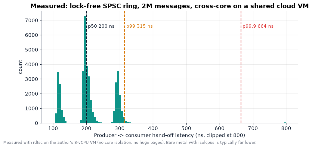
The median cross-core hand-off is roughly 200-250 ns on a shared VM with no core isolation. The p99.9 tail and the occasional very large maximum come from hypervisor and scheduler preemption, not from the queue. On a pinned, isolated bare-metal core the same code typically runs in the tens of nanoseconds. The structure is what matters: no locks, no CAS loops, acquire/release ordering only, and cached indices.
8.2 Cache-aligned L2 book with fixed-point microprice
Here the price ladder is a flat array indexed by tick − base, masked to a power of two, so an update is a single indexed store and never touches a tree or hash map. Imbalance is computed in Q15 fixed point and the microprice in integer nano-units, with no floating point on the hot path.
// l2_book.cpp -- cache-aligned, array-indexed L2 price ladder with fixed-point prices
// and branch-light imbalance / microprice. g++ -O3 -std=c++20
#include <array>
#include <cstdint>
#include <cstdio>
#include <chrono>
#include <random>
#include <bit>

using Px = int64_t;                         // price in ticks (fixed point)
constexpr int64_t kTickNano = 250'000'000;  // 0.25 index points in 1e-9 units (MES/ES)

template <int Levels>
struct alignas(64) Ladder {                 // sizes indexed by (tick - base)
    static_assert(std::has_single_bit(unsigned(Levels)));
    Px base = 0;
    alignas(64) std::array<int32_t, Levels> qty{};
    int32_t& at(Px tick) { return qty[size_t(tick - base) & (Levels - 1)]; }
};

struct alignas(64) Book {
    Ladder<4096> bids, asks;
    Px best_bid = 0, best_ask = 0;

    void set_bid(Px t, int32_t q) {
        bids.at(t) = q;
        if (q > 0 && t > best_bid) best_bid = t;
        else if (q == 0 && t == best_bid) while (best_bid > bids.base && bids.at(best_bid) == 0) --best_bid;
    }
    void set_ask(Px t, int32_t q) {
        asks.at(t) = q;
        if (q > 0 && (best_ask == 0 || t < best_ask)) best_ask = t;
        else if (q == 0 && t == best_ask) while (best_ask < asks.base + 4095 && asks.at(best_ask) == 0) ++best_ask;
    }
    // Imbalance in Q15 fixed point: (b - a) / (b + a) * 32768, no floating point
    int32_t imbalance_q15(Px bb, Px ba) {
        const int64_t b = bids.at(bb), a = asks.at(ba);
        const int64_t s = b + a;
        return int32_t(((b - a) << 15) / (s + (s == 0)));     // branch-free divide guard
    }
    // Microprice in 1e-9 units: ask*I + bid*(1-I), I = b/(b+a); integer only
    int64_t microprice_nano() {
        const int64_t b = bids.at(best_bid), a = asks.at(best_ask);
        const int64_t s = b + a + (b + a == 0);
        const int64_t bid = best_bid * kTickNano, ask = best_ask * kTickNano;
        return bid + ((ask - bid) * b) / s;
    }
};

int main() {
    static Book bk;
    const Px mid = 7585'00 / 25;            // 7585.00 / 0.25 = 30340 ticks
    bk.bids.base = bk.asks.base = mid - 2048;
    for (int i = 1; i <= 20; ++i) { bk.set_bid(mid - i + 1, 50 + i * 5); bk.set_ask(mid + i, 40 + i * 7); }

    std::mt19937_64 rng(42);
    constexpr int kUpd = 20'000'000;
    int64_t chk = 0;
    auto t0 = std::chrono::steady_clock::now();
    for (int i = 0; i < kUpd; ++i) {
        const uint64_t r = rng();
        const int lvl = int(r & 7);
        const int32_t q = int32_t((r >> 8) & 255);           // 0 => level cleared
        if (r & (1ull << 40)) bk.set_bid(bk.best_bid - lvl, q + (lvl == 0));
        else                  bk.set_ask(bk.best_ask + lvl, q + (lvl == 0));
        chk += bk.imbalance_q15(bk.best_bid, bk.best_ask) + (bk.microprice_nano() & 1023);
    }
    auto ns = std::chrono::duration<double, std::nano>(std::chrono::steady_clock::now() - t0).count();
    std::printf("updates=%d  ns/update(incl. imbalance+microprice)=%.2f  checksum=%lld\n",
                kUpd, ns / kUpd, (long long)chk);
    std::printf("best bid %.2f x %d | best ask %.2f x %d | I=%.4f | micro=%.6f\n",
                bk.best_bid * 0.25, bk.bids.at(bk.best_bid), bk.best_ask * 0.25, bk.asks.at(bk.best_ask),
                bk.imbalance_q15(bk.best_bid, bk.best_ask) / 32768.0, bk.microprice_nano() * 1e-9);
}
Measured output:
updates=20000000  ns/update(incl. imbalance+microprice)=10.81  checksum=10148154517
best bid 7585.00 x 131 | best ask 7585.25 x 160 | I=-0.0996 | micro=7585.112543
About 11 ns per book update, including recomputing imbalance and microprice, with a random-number generator in the loop. The (s == 0) trick in the division guard is a typical branch-free idiom. It adds 1 to the denominator only when the queue is empty, which avoids a divide-by-zero without a branch.
8.3 Structure-of-arrays Black-76 for a whole chain
This reprices a 4,096-strike chain in one pass. It uses a structure-of-arrays layout, a branch-light normal CDF (Abramowitz-Stegun 26.2.17, absolute error below 7.5e-8) and put-call parity to get puts nearly for free. This is how you’d refresh model values for every strike on every futures tick.
// black76_batch.cpp -- structure-of-arrays Black-76 pricer + delta/vega for a whole
// options-on-futures chain, with a fast normal CDF. g++ -O3 -std=c++20 [-march=native]
#include <cmath>
#include <cstdio>
#include <vector>
#include <chrono>
#include <algorithm>

// Abramowitz-Stegun 26.2.17 (|err| < 7.5e-8): branch-light, auto-vectorisable
static inline double ncdf_fast(double x) {
    const double ax = std::fabs(x);
    const double t = 1.0 / (1.0 + 0.2316419 * ax);
    const double poly = t * (0.319381530 + t * (-0.356563782 + t * (1.781477937
                       + t * (-1.821255978 + t * 1.330274429))));
    const double tail = 0.3989422804014327 * std::exp(-0.5 * ax * ax) * poly;
    return x >= 0.0 ? 1.0 - tail : tail;              // compiles to a blend, not a jump
}
static inline double ncdf_ref(double x) { return 0.5 * std::erfc(-x * M_SQRT1_2); }

struct Chain {                                         // SoA layout: contiguous per field
    std::vector<double> K, sigma, call, put, delta_c, vega;
    explicit Chain(size_t n) : K(n), sigma(n), call(n), put(n), delta_c(n), vega(n) {}
};

template <double (*N)(double)>
void price_chain(Chain& c, double F, double T, double r) {
    const double df = std::exp(-r * T), sqT = std::sqrt(T);
    const size_t n = c.K.size();
    for (size_t i = 0; i < n; ++i) {
        const double sq = c.sigma[i] * sqT;
        const double d1 = (std::log(F / c.K[i]) + 0.5 * sq * sq) / sq;
        const double d2 = d1 - sq;
        const double n1 = N(d1), n2 = N(d2);
        c.call[i]    = df * (F * n1 - c.K[i] * n2);
        c.put[i]     = c.call[i] - df * (F - c.K[i]);  // put-call parity on futures
        c.delta_c[i] = df * n1;
        c.vega[i]    = df * F * sqT * 0.3989422804014327 * std::exp(-0.5 * d1 * d1);
    }
}

int main() {
    const double F = 7585.12, T = 38.0 / 365.0, r = 0.045;   // ES ref + 38 DTE + 4.5%
    const size_t n = 4096;
    Chain a(n), b(n);
    for (size_t i = 0; i < n; ++i) {                          // strikes 6000..9000, skewed vol
        const double K = 6000.0 + 3000.0 * double(i) / double(n - 1);
        const double k = std::log(K / F);
        const double vol = 0.14 - 0.25 * k + 0.6 * k * k;     // ILLUSTRATIVE smile
        a.K[i] = b.K[i] = K; a.sigma[i] = b.sigma[i] = vol;
    }
    auto bench = [&](auto fn, Chain& c) {
        const int reps = 2000;
        auto t0 = std::chrono::steady_clock::now();
        for (int k = 0; k < reps; ++k) { fn(c, F, T, r); asm volatile("" ::: "memory"); }
        return std::chrono::duration<double, std::nano>(std::chrono::steady_clock::now() - t0).count()
               / (double(reps) * double(n));
    };
    const double ns_fast = bench(price_chain<ncdf_fast>, a);
    const double ns_ref  = bench(price_chain<ncdf_ref>,  b);
    double max_err = 0.0;
    for (size_t i = 0; i < n; ++i) max_err = std::max(max_err, std::fabs(a.call[i] - b.call[i]));
    const size_t atm = size_t(double(n - 1) * (F - 6000.0) / 3000.0);
    std::printf("ns/option: fast-CDF=%.2f  erfc-CDF=%.2f  speed-up=%.2fx\n", ns_fast, ns_ref, ns_ref / ns_fast);
    std::printf("max |call price error| = %.3e index points over %zu strikes\n", max_err, n);
    std::printf("ATM-ish K=%.2f vol=%.4f call=%.4f put=%.4f delta=%.4f vega=%.3f\n",
                a.K[atm], a.sigma[atm], a.call[atm], a.put[atm], a.delta_c[atm], a.vega[atm]);
}
Measured output:
ns/option: fast-CDF=31.11  erfc-CDF=37.69  speed-up=1.21x
max |call price error| = 6.737e-04 index points over 4096 strikes
ATM-ish K=7584.62 vol=0.1400 call=136.3060 put=135.8038 delta=0.5072 vega=971.533
About 30 ns per option for call, put, delta and vega together, with a maximum price error of about 7e-4 index points against the erfc reference. That’s $0.03 on an ES contract, and much less than one tick. The speed-up is modest because log and exp dominate. To go further, compile with -O3 -march=native -ffast-math so glibc’s vector math library can SIMD the transcendental functions, or precompute ln(K) per strike and update only ln(F) per tick.
8.4 O(1) risk engine and a branch-free pre-trade gate
This keeps running statistics (Welford mean and variance, EWMA variance, running peak-to-trough drawdown) and runs a pre-trade check that returns a bitmask of violations instead of branching early. The bitmask makes every check cost the same time, and the bits tell you which limit tripped. As a cross-check, it replays the ZN bot’s 12 trades from the PDF.
// risk_engine.cpp -- O(1)-per-event risk state: Welford mean/variance, EWMA vol,
// running drawdown, and a branch-light pre-trade gate. g++ -O3 -std=c++20
#include <cmath>
#include <cstdint>
#include <cstdio>
#include <chrono>

struct alignas(64) RunningStats {          // Welford: numerically stable, one pass
    uint64_t n = 0; double mean = 0, m2 = 0, ewma_var = 0, lam = 0.94;
    double equity = 0, peak = 0, max_dd = 0, peak_at_max_dd = 0;
    void add(double x) {
        ++n; const double d = x - mean; mean += d / double(n); m2 += d * (x - mean);
        ewma_var = (n == 1) ? x * x : lam * ewma_var + (1 - lam) * x * x;
        equity += x;
        const double new_peak = equity > peak ? equity : peak;   // compiles to maxsd
        peak = new_peak;
        const double dd = peak - equity;
        const bool worse = dd > max_dd;
        max_dd = worse ? dd : max_dd;
        peak_at_max_dd = worse ? peak : peak_at_max_dd;
    }
    double var() const { return n > 1 ? m2 / double(n - 1) : 0.0; }
    double sharpe_per_event() const { const double v = var(); return v > 0 ? mean / std::sqrt(v) : 0; }
};

struct Limits { int64_t max_pos, max_order_qty; int64_t band_ticks; double daily_loss_limit; };

// Returns a bitmask of violated checks (0 == pass). No early returns => predictable timing.
static inline uint32_t pretrade(const Limits& L, int64_t pos, int64_t qty, int64_t px_ticks,
                                int64_t ref_ticks, double day_pnl, bool kill) {
    const int64_t new_pos = pos + qty;
    const int64_t dev = px_ticks > ref_ticks ? px_ticks - ref_ticks : ref_ticks - px_ticks;
    uint32_t m = 0;
    m |= uint32_t((new_pos > L.max_pos) | (new_pos < -L.max_pos)) << 0;
    m |= uint32_t((qty > L.max_order_qty) | (qty < -L.max_order_qty)) << 1;
    m |= uint32_t(dev > L.band_ticks) << 2;                       // fat-finger price band
    m |= uint32_t(day_pnl <= -L.daily_loss_limit) << 3;           // daily loss circuit breaker
    m |= uint32_t(kill) << 4;                                     // manual kill switch
    return m;
}

int main() {
    // Replay the 12 ZN trade P&Ls printed in the backtest PDF (USD)
    const double zn[] = {-2193.08, 4051.34, -1824.78, 3515.62, 5558.04, 6406.25, 8906.25,
                         5156.25, -3532.37, -3867.19, -4068.08, -3498.88};
    RunningStats s; s.equity = s.peak = 15000.0;                  // $15,000 starting capital
    for (double x : zn) s.add(x);
    std::printf("n=%llu mean=%.2f sd=%.2f SR/trade=%.3f maxDD=$%.2f (%.1f%% of peak equity %.2f)\n",
                (unsigned long long)s.n, s.mean, std::sqrt(s.var()), s.sharpe_per_event(),
                s.max_dd, 100.0 * s.max_dd / s.peak_at_max_dd, s.peak_at_max_dd);

    const Limits L{5, 2, 40, 750.0};
    std::printf("gate(ok)=%u gate(oversize)=%u gate(fat-finger)=%u gate(loss-limit)=%u\n",
                pretrade(L, 1, 1, 30340, 30338, -100, false), pretrade(L, 4, 3, 30340, 30338, -100, false),
                pretrade(L, 0, 1, 30500, 30338, -100, false), pretrade(L, 0, 1, 30340, 30338, -800, false));
    // micro-benchmark the gate
    constexpr int kN = 100'000'000; uint32_t acc = 0;
    auto t0 = std::chrono::steady_clock::now();
    for (int i = 0; i < kN; ++i)
        acc += pretrade(L, i & 7, (i & 3) - 1, 30338 + (i & 63), 30338, -double(i & 1023), false);
    const double ns = std::chrono::duration<double, std::nano>(std::chrono::steady_clock::now() - t0).count();
    std::printf("pre-trade gate: %.3f ns/check (acc=%u)\n", ns / kN, acc);
}
Measured output:
n=12 mean=1217.45 sd=4797.64 SR/trade=0.254 maxDD=$14966.52 (33.6% of peak equity 44575.89)
gate(ok)=0 gate(oversize)=3 gate(fat-finger)=4 gate(loss-limit)=8
pre-trade gate: 1.407 ns/check (acc=382811952)
The C++ replay matches the Python: mean $1,217.45, standard deviation $4,797.64 and a maximum drawdown of $14,966.52, which is 33.6% of $44,575.89 peak equity rather than the PDF’s 99.8%. The gate costs 1-2 ns per check, which is cheap enough to run on every order. The limits shown (position cap, order-size cap, price band, daily-loss circuit breaker and kill switch) are generic exchange-style controls, not any bot’s strategy logic.
9. Data-integrity audit: sixteen things to fix before any of this touches capital
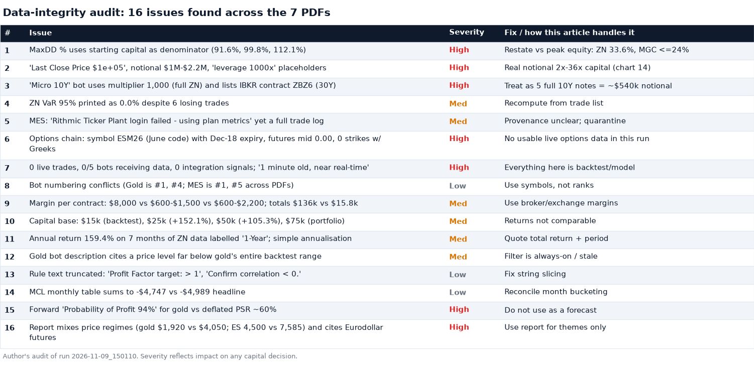
The severe items share a theme: the numbers look precise, but nobody has checked what they’re measuring. A drawdown divided by the wrong base, a leverage line that’s a placeholder, a “micro” contract that’s full size, a chain with a June symbol and a December expiry, and a “near real-time” stamp on a feed that never connected. None of these changes which bots made money. All of them change how much you’d risk, and that’s where accounts get hurt.
Here’s what I’d fix first, in order:
Drawdown denominator. Report drawdown against peak equity. Keep “% of starting capital” as a separate ruin metric.
Contract master. Use one table for root, multiplier, tick value and exchange margin, read by every report. That would fix the ZN/ZB/micro confusion, the 1000x leverage line and the three-way margin disagreement in one place.
Data-health gating. If zero bots are receiving data, the options and signal pages should say “NO DATA” rather than “1 minute old”. The MES backtest should fail loudly if its data source failed.
One capital base. Use $15k per bot or $75k per book, not $25k or $50k in different PDFs.
Deflated statistics. Print the PSR and deflated Sharpe next to every Sharpe, and drop the “forward probability of profit” until it’s computed out of sample.
Narrative levels. Have the report generator pull current futures settlements and reject strikes more than about 30% from them. That would have caught gold strikes of 1,800-2,300 against a $4,050 market.
10. The playbook, in one place
What the evidence supports:
Core view 1: long gold, defined risk. The 4100/4300 call debit spread (R:R 2.80) or the zero-cost 3900/3700 vs 4200/4400 spread collar. Size it to about one-tenth Kelly of the bot’s edge, and stop if the bot’s trailing 20-trade P&L keeps falling. It was ‑$5,682 in the latest 20.
Core view 2: short duration, defined risk. The ZN 108/106 put spread (R:R 1.39) instead of a 36x-levered outright short into a crowded 450K-contract CTA position. CPI on November 10 is the first test.
Tail hedges. The ES 7000/6800 put spread ($206 for up to $9,793) and the VIX 25/30 call spread ($879 for up to $4,117). Together they cost about 5% of the risk budget and pay in the scenario that hurts both core views.
Research, not capital. The Brent-WTI widening and CL backwardation trades (freight-driven), and the MNQ bot sitting on its breakeven line.
Avoid. Short ZN with the report’s 110/115 call-spread hedge (open-ended above 115), the NatGas short strangle (open-ended tails at 60% IV), and the MCL and MES bots.
What would change my mind:
A live, gateway-connected run where the options chain returns real strikes. Then the skew metrics, the true 25-delta risk reversal and live Greeks replace my flat-vol prices.
Gold’s trailing trades turning positive again, or out-of-sample months that look like January and August 2026.
More than about 30 ZN trades with a per-trade t-stat above 2.
A soft CPI that squeezes the duration short. That would test whether the ZN thesis is a trend or a crowded trade.
The meta-lesson. This run produced a lot of confident numbers: 407 rules, Sharpe ratios to three decimals and a 94% probability of profit. When you strip it back to what can be verified, what’s left is two plausible macro bets, one statistically detectable but concentrated edge, and a long list of reporting bugs. That’s still a useful result. The goal is to find out what you actually know before the market does it for you.
Disclaimer. Educational research only, not investment advice. All bot results are hypothetical backtests on historical four-hour data. They don’t reflect slippage, actual fills or live trading, and they are not indicative of future results. Options prices are model outputs (Black-76, flat volatility), with inputs either cited from the source PDFs or marked as assumptions. Narrative market levels and positioning figures are reproduced as cited by an automated report and have not been independently verified. Futures and options carry a substantial risk of loss, including losses beyond your initial margin. Consult a qualified professional before making any trading decision.