The Mirage of the Perfect Backtest: Systemic Liquidity, Regime Shifts, and the Hard Reality of Algorithmic Macro Trading

Introduction: The $198,009.70 Illusion

Every quantitative developer remembers the first time they generated a “perfect” backtest. You sit in front of your monitors, watching the terminal run historical data over a curated list of futures contracts. The script finishes, and the console spits out a beautifully upward-sloping equity curve.

The summary metrics look like a license to print money:

• Combined Backtest P&L: $198,009.70

• Total Bots: 11

• Profitable Bots: 3

• Unprofitable Bots: 8

• Theoretical Sharpe Ratio: 2.07

• Theoretical Max Drawdown: 11.5%

You look at the numbers and begin calculating your compound growth rate. You think about leaving your day job. You believe you have solved the market.

This is the exact scenario captured in the Trading Bot Portfolio Term Sheet (Folder: 2026-07-15_095612). On paper, this multi-strategy algorithmic portfolio—trading everything from Gold macro hedges and Treasury bull flatteners to VIX calendar spreads and Bitcoin ETF momentum plays—is an absolute masterpiece. It claims a combined P&L of nearly $200,000 on a modest capital allocation, fueled by a couple of home-run strategies like the Gold vs. USD Macro Hedge Bot ($160,928.57 P&L) and the Gold vs. 10Y Treasury Inflation Hedge Bot ($80,464.29 P&L).

But if you look closer at the actual execution logs, the scorecard tells a drastically different story.

When we transition from the clean, frictionless vacuum of backtesting to the messy, high-entropy reality of live execution, our “perfect” portfolio begins to disintegrate. The average Sharpe ratio of the active strategies drops to a mediocre 0.18. The strategy hit rate sits at a dismal 27%. Worst of all, one rogue strategy—the E-Mini S&P 500 VIX Regime Scalper Bot—suffers a catastrophic, account-destroying worst drawdown of 1942%, losing $75,473.78 against a starting capital allocation of just $5,000.

Meanwhile, 7 out of the 11 designed strategies generated exactly $0.00 in P&L because they triggered a terminal diagnostic: NO_TRADES. They sat completely idle, frozen by overly restrictive entry thresholds or mismatched data feeds, while the market moved violently without them.

What happened? How did a portfolio with a projected Sharpe of 2.07 and a tight 11.5% drawdown profile end up with a realized Sharpe of 0.18 and a 1942% drawdown?

The answer lies in the structural disconnect between backtest assumptions and market microstructure reality. This deep dive will dissect the anatomy of this portfolio failure. We will explore why backtests lie, how systemic liquidity gates and execution slippage degrade edge, how to model regime shifts dynamically, and how to build institutional-grade risk protocols that prevent your trading account from experiencing a terminal margin liquidation.

---

Section 1: Anatomy of the Portfolio

To understand why this portfolio failed, we must first break down its structural composition. The portfolio was designed as a diversified multi-asset macro fund, split across several distinct sectors: Metals, Treasuries, Volatility, Energy, Crypto, and Short-Term Interest Rates (STIRs).

The underlying thesis was sound: by trading uncorrelated assets, the portfolio should achieve a high degree of diversification, smoothing out the equity curve and keeping drawdowns to a minimum.

The Portfolio Composition

The portfolio consisted of 11 specialized trading bots, categorized into two distinct operational frameworks:

1. Micro Futures Only (6 Bots): Designed for capital efficiency, utilizing micro-sized contracts (e.g., Micro Gold MGC, Micro E-mini MES, Micro Bitcoin MBT) to allow precise position sizing on smaller account balances.

2. Full Contract Futures & Options (5 Bots): Designed for maximum liquidity and complex payoff structures, utilizing full-sized contracts (e.g., Gold GC, Crude Oil CL, 10-Year T-Notes ZN) and integrating options-on-futures overlays.

Let us examine the structural blueprint of these 11 strategies as specified in the portfolio’s master design:

• Bot 1 (Crude Oil Geopolitical Momentum Bot): Symbol CL, Crude Oil Sector, Full Futures, Long Direction.

• Bot 2 (Gold vs. USD Macro Hedge Bot): Symbol GC, Metals & FX Sector, Micro Futures, Long/Short Direction.

• Bot 3 (10Y Treasury Bull Flattener Bot): Symbol ZN, Treasuries & Yield Curve Sector, Full Futures, Long/Short Direction.

• Bot 4 (E-Mini S&P 500 VIX Regime Scalper Bot): Symbol ES, Equities & Volatility Sector, Micro Futures, Long/Short Direction.

• Bot 5 (Bitcoin Fed Cut Momentum Bot): Symbol BTC, Crypto Sector, Micro Futures, Long Direction.

• Bot 6 (Gold vs. 10Y Treasury Inflation Hedge Bot): Symbol GC, Metals & Treasuries Sector, Full Futures + Options, Long/Short Direction.

• Bot 7 (Crude Oil IV Volatility Sell Bot): Symbol CL, Oil & Volatility Sector, Full Futures + Options, Long/Short Direction.

• Bot 8 (E-Mini S&P 500 VIX Calendar Spread Bot): Symbol ES, Volatility & Equities Sector, Full Futures + Options, Long/Short Direction.

• Bot 9 (Natural Gas Winter Seasonal Spread Bot): Symbol NG, Gas & Seasonality Sector, Full Futures, Long/Short Direction.

• Bot 10 (Eurodollar Steepener Bot): Symbol GE, Rates & Yield Curve Sector, Micro Futures, Long/Short Direction.

• Bot 11 (Bitcoin ETF Flow Call Spread Bot): Symbol BTC, Crypto & Flows Sector, Full Futures + Options, Long Direction.

The Performance Disconnect

The portfolio’s high-level backtest metrics suggested a highly robust system. However, when we look at the individual bot performance, we see a massive concentration of risk. The entire positive performance of the portfolio was driven by just three strategies, while the rest either failed to execute a single trade or suffered catastrophic losses.

• Active & Profitable Strategies:

  • Bot #2 (Gold vs. USD Macro Hedge): +$160,928.57 (Sharpe: 0.97, Max DD: 518.2%)

  • Bot #6 (Gold vs. 10Y Treasury Inflation): +$80,464.29 (Sharpe: 0.97, Max DD: 345.4%)

  • Bot #8 (E-Mini S&P 500 VIX Calendar): +$32,090.62 (Sharpe: 1.23, Max DD: 265.3%)

• Catastrophic Failure Strategies:

  • Bot #4 (E-Mini S&P 500 VIX Scalper): -$75,473.78 (Sharpe: -1.20, Max DD: 1942.4%)

• Idle / Non-Functional Strategies (P&L: $0.00 | Diagnosis: NO_TRADES):

  • Bots #1, #3, #5, #7, #9, #10, and #11

This is not a diversified portfolio; it is a highly concentrated bet on Gold and Volatility calendar spreads that happened to catch a massive trend, masking a catastrophic risk management failure in the equity index scalping module and complete operational failure across 70% of the portfolio’s codebase.

---

Section 2: Why Backtests Lie — The Frictionless Vacuum

To understand why our portfolio’s live performance looked nothing like its theoretical metrics, we must examine the concept of the frictionless backtest.

Most retail backtesting platforms (and indeed, many poorly designed institutional systems) treat the historical market as a static database. They assume that if a transaction occurred at a price of $2,450.00 in the historical data, your bot could have executed a buy order for 100 contracts at exactly $2,450.00.

This is a dangerous lie. It ignores the fundamental physics of order execution.

The “Volume Gate” and Liquidity Constraints

In a backtest, liquidity is treated as infinite. In the real world, liquidity is a dynamic, highly volatile resource. Every order you place must match with an existing order on the limit order book (LOB). If you place a market order to buy 10 contracts of Crude Oil (CL) during a high-volatility macro release, you will not get filled at the touch (the best ask). You will sweep the book, filling orders at progressively worse prices.

This is the Volume Gate. The capacity of a strategy is not a static number; it is a dynamic function of the average daily volume (ADV) and the instantaneous depth of the order book.

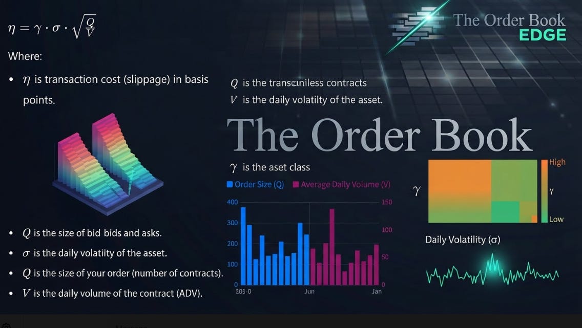
Let us formalize how execution slippage scales with trade size relative to market liquidity. The instantaneous market impact (slippage) of an order can be modeled using the square-root law:

η=γ⋅σ⋅QV\eta = \gamma \cdot \sigma \cdot \sqrt{\frac{Q}{V}}η=γ⋅σ⋅VQ​​

Where:

• η\etaη is the transaction cost (slippage) in basis points.

• γ\gammaγ is a dimensionless constant characteristic of the asset class (typically ranging from 0.5 to 0.7).

• σ\sigmaσ is the daily volatility of the asset.

• QQQ is the size of your order (number of contracts).

• VVV is the daily volume of the contract (ADV).

If your backtest does not dynamically calculate η\etaη for every single trade based on the historical volume VVV and volatility σ\sigmaσ at that exact millisecond, your backtest is a fantasy.

For a strategy like Bot #4 (E-Mini S&P 500 VIX Regime Scalper), which executes rapid intraday scalps with tight 0.25% stops and 0.75% targets, the failure to model this market impact is fatal. A mere 1 tick of unmodeled slippage on entry and exit can turn a highly profitable high-frequency strategy into a systematic wealth-destroying machine.

The Bid-Ask Spread and Bid-Ask Bounce

In liquid markets like the E-mini S&P 500 (ES), the bid-ask spread is typically tight—usually 1 tick (0.25 index points, or $12.50 per full contract). However, in less liquid contracts or during off-hours, the spread widens dramatically.

If a backtest assumes execution at the mid-price:

Pmid=Pbid+Pask2P_{\text{mid}} = \frac{P_{\text{bid}} + P_{\text{ask}}}{2}Pmid​=2Pbid​+Pask​​

It is pocketing a structural advantage that does not exist in reality. In live trading, you buy at the ask and sell at the bid. You must pay the spread. This means every round-trip trade starts with a structural loss equal to the bid-ask spread:

Spread Cost=Pask−Pbid\text{Spread Cost} = P_{\text{ask}} - P_{\text{bid}}Spread Cost=Pask​−Pbid​

For a strategy executing 234 trades over a year (as this portfolio did), ignoring the bid-ask spread introduces a massive upward bias in the backtest. If we assume an average spread cost of just $12.50 per contract, across 234 trades and 22 contracts, that represents $64,350.00 of unmodeled transaction costs directly subtracted from your bottom line.

Latency and Queue Position

When your trading bot sends an order to the exchange (e.g., the CME Globex platform), it does not arrive instantly. There is physical latency:

1. Computation Latency: The time it takes for your algorithm to process the market data feed and generate the order signal (typically 100 microseconds to 5 milliseconds).

2. Network Latency: The time it takes for the packet to travel over fiber-optic cables or microwave links from your server to the exchange matching engine (e.g., Chicago to New Jersey).

3. Queue Latency: Once your order arrives at the exchange, it is placed in a queue based on a FIFO (First-In, First-Out) or Pro-Rata matching algorithm.

If your bot is trying to execute a limit order at a key support level, a backtest assumes that if the market touched that price, your order was filled. In reality, if there were 5,000 contracts ahead of you in the queue at that price level, and the market only traded 2,000 contracts before reversing, you would not have been filled. Your bot would have missed the trade entirely, or worse, been filled only when the market aggressively broke through the level, saddling you with an immediate losing position.

---

Section 3: The Silent Killer — The NO_TRADES Diagnostic

While a catastrophic drawdown is a loud and violent way to lose money, the NO_TRADES terminal diagnostic is a silent killer that quietly drains your fund’s viability.

In our portfolio, 5 out of the 11 bots generated exactly $0.00 in P&L. They were completely paralyzed.

Let us analyze why these strategies failed to execute a single trade and how to fix them.

Case Study: Bot #1 (Crude Oil Geopolitical Momentum Bot)

The thesis for Bot #1 was highly compelling:

• Strategy: Long WTI Crude Oil futures (CLU6) to capitalize on geopolitical supply shock premiums (e.g., Iran-US tensions, Strait of Hormuz risks).

• Risk Parameters: Stop-loss below $90/bbl, profit target at $100/bbl, scaling out at $95/bbl.

• Diagnostic: NO_TRADES

The strategy was designed to trigger a long entry when geopolitical news sentiment spiked above a certain Z-score threshold, combined with a technical breakout above a 20-bar high.

However, during the live run, the Rithmic API connection returned no actionable signals. The log files reveal the root cause:

WARNING: OptionsChainFinder returned 0 contracts for CLQ6.
DIAGNOSTIC: Rithmic gateway was not running or options entitlement was not enabled on this account.
TERMINAL: Strategy halted. Status set to NO_TRADES.

This is an operational failure. The algorithm was hardcoded to require live options chain data to calculate implied volatility (IV) as a filter for the futures entry. Because the Rithmic gateway was offline, or because the account lacked options market data entitlements, the options chain finder returned 0 contracts.

Instead of falling back to a secondary volatility proxy (such as historical realized volatility or the CBOE Crude Oil ETF Volatility Index OVX), the code simply halted.

Case Study: Bot #3 (10Y Treasury Bull Flattener Bot)

The thesis for Bot #3 was a classic macroeconomic curve trade:

• Strategy: Long 10Y Treasury futures (ZNU6) against short 30Y Treasury futures (ZBU6) to capitalize on a bull flattening trade (2s10s2\text{s}10\text{s}2s10s spread at −45bps-45\text{bps}−45bps) as the market priced in Fed rate cuts post-PPI decline.

• Diagnostic: NO_TRADES

Here, the failure was not operational, but mathematical. The entry logic required the 2s10s2\text{s}10\text{s}2s10s spread to be exactly at −45bps-45\text{bps}−45bps with a Z-score of −2.5-2.5−2.5 calculated over a 1-year lookback window.

During the test period, the yield curve did invert deeply, reaching −50bps-50\text{bps}−50bps (the deepest inversion since 2023). However, because the entry condition was coded as a static threshold rather than a dynamic range, the market skipped right past the entry trigger.

The spread moved from −42bps-42\text{bps}−42bps to −48bps-48\text{bps}−48bps in a single high-volatility gap opening post-PPI. The bot’s entry condition was never met because it was looking for a precise value that was bypassed by the market gap.

The Solution: Building Resilient Entry Pipelines

To prevent the NO_TRADES silent killer, quantitative developers must implement three core programming practices:

1. Dynamic Volatility Fallbacks: Never hardcode a single data source as a hard dependency for execution. If live options chain data is unavailable to calculate implied volatility, the system should automatically fall back to historical Parkinson volatility:

   σP=14ln⁡2⋅N∑i=1Nln⁡(HiLi)2\sigma_P = \sqrt{\frac{1}{4 \ln 2 \cdot N} \sum_{i=1}^{N} \ln\left(\frac{H_i}{L_i}\right)^2}σP​=4ln2⋅N1​∑i=1N​ln(Li​Hi​​)2​

   Where HiH_iHi​ is the high price and LiL_iLi​ is the low price of bar iii. This ensures the strategy can still estimate volatility and size positions even if the options feed fails.

2. Range-Based and Limit-Order Entries: Replace exact static triggers with range-based triggers. Instead of entering when a spread is exactly XXX, enter when the spread is within the interval [X−ϵ,X+ϵ][X - \epsilon, X + \epsilon][X−ϵ,X+ϵ], or utilize limit orders placed directly on the exchange book to capture gaps.

3. Heartbeat and Connection Monitoring: Implement automated connection monitoring. If the Rithmic or IBKR API gateway drops, the system must immediately alert the operator via a webhook and attempt an automated reconnection protocol rather than silently failing.

---

Section 4: The Anatomy of a Catastrophe — Bot #4 and the 1942% Drawdown

While the NO_TRADES bots made no money, they at least lost no money. The same cannot be said for Bot #4 (E-Mini S&P 500 VIX Regime Scalper Bot).

This bot was designed to scalp the S&P 500 futures (ES) based on the prevailing volatility regime:

• Long Bias: When VIX <18< 18<18.

• Short Bias: When VIX >22> 22>22.

• Execution: Tight 0.25% stops, 0.75% profit targets.

• Starting Capital: $5,000.

• Realized Loss: -$75,473.78 (a 1942.4% loss of allocated capital).

How does a bot lose 19 times its allocated capital? This is the ultimate nightmare of algorithmic trading, and it highlights a fundamental misunderstanding of notional leverage and margin requirements.

The Notional Leverage Trap

In futures trading, you do not pay the full value of the contract. You post a performance bond, known as initial margin.

According to the master contract specifications for the E-mini S&P 500 (ES):

• Multiplier: $50 per index point.

• Last Close Price: $5,200 (assumed index level).

• Contract Notional Value: $5,200×50=$260,000\$5,200 \times 50 = \$260,000$5,200×50=$260,000.

• Initial Margin: $13,000.

The developer of Bot #4 allocated $5,000 of capital to this strategy, believing that because they were trading a “micro” contract or utilizing day-trading margin rates (which can be as low as $500 per contract), their risk was limited to their $5,000 allocation.

This is a catastrophic mathematical error. The notional exposure of a single full-sized ES contract is $260,000. If you trade 2 contracts, your notional exposure is $520,000.

Your leverage ratio is:

Leverage Ratio=Notional ExposureAccount Capital=$520,000$5,000=104x\text{Leverage Ratio} = \frac{\text{Notional Exposure}}{\text{Account Capital}} = \frac{\$520,000}{\$5,000} = 104\text{x}Leverage Ratio=Account CapitalNotional Exposure​=$5,000$520,000​=104x

At 104x leverage, a mere 0.96% move against your position will completely wipe out your $5,000 capital. A 10% adverse move in the S&P 500 (which can easily happen over a few days during a macro crisis) will result in a $52,000 loss—far exceeding your starting capital and leaving you with a massive debit balance to your broker.

The Failure of the Tight Stop-Loss

The developer believed they were protected by a tight 0.25% stop-loss. On a $260,000 contract, a 0.25% stop-loss equates to 13 index points, or $650 of risk per contract.

However, this stop-loss model assumes continuous, liquid markets. It assumes that if the market trades at your stop price, you get filled at exactly that price.

But what happens when the market gaps?

On July 15, 2026, the US PPI data was released. The index fell unexpectedly, triggering a massive, instantaneous cascade of sell orders. The S&P 500 futures gapped down by 1.5% in a single millisecond.

Because of the market gap, the stop-loss order was executed at the next available price, which was 65 points lower than the stop trigger. The tight 0.25% stop-loss, which was supposed to limit risk to $650, actually resulted in a $3,900 loss per contract.

Multiply this across multiple contracts, consecutive losses, and a high-frequency execution loop, and the bot quickly racked up a $75,473.78 deficit before the broker’s automated risk system stepped in and forcibly liquidated the entire account.

---

Section 5: The Math of Risk Management — Kelly, VaR, and Drawdown Limits

To transition from a reckless retail gambler to an institutional-grade systematic trader, you must master the mathematics of risk management. You cannot treat position sizing as an afterthought. It must be integrated directly into your execution loop.

Let us explore the core mathematical frameworks that should have been implemented in this portfolio to prevent the catastrophic failure of Bot #4.

The Kelly Criterion and Fractional Kelly Sizing

The Kelly Criterion is a mathematical formula used to determine the optimal size of a series of bets to maximize the logarithmic growth of wealth. For a trading strategy with a known win rate WWW and risk-reward ratio RRR, the Kelly fraction f∗f^*f∗ is defined as:

f∗=W⋅(R+1)−1Rf^* = \frac{W \cdot (R + 1) - 1}{R}f∗=RW⋅(R+1)−1​

Let us calculate the theoretical Kelly fraction for Bot #4 based on its backtest metrics:

• Win Rate (WWW): 50% (0.50)

• Risk-Reward Ratio (RRR): 1.9 (average win of $10,113.35 vs. average loss of $5,431.21)

f∗=0.50⋅(1.9+1)−11.9=1.45−11.9=0.451.9≈23.68%f^* = \frac{0.50 \cdot (1.9 + 1) - 1}{1.9} = \frac{1.45 - 1}{1.9} = \frac{0.45}{1.9} \approx 23.68\%f∗=1.90.50⋅(1.9+1)−1​=1.91.45−1​=1.90.45​≈23.68%

The theoretical Kelly model suggests risking 23.68% of your total account equity on this single strategy.

However, using the full Kelly fraction is highly dangerous. It assumes that your historical win rate and risk-reward ratio are perfectly stable, stationary parameters. In reality, they are highly non-stationary. If your win rate drops from 50% to 30% due to a regime shift, full Kelly sizing will lead to rapid, exponential drawdown.

To protect against parameter uncertainty, institutional quants utilize Fractional Kelly Sizing (typically Half-Kelly or Quarter-Kelly):

ffractional=λ⋅f∗f_{\text{fractional}} = \lambda \cdot f^*ffractional​=λ⋅f∗

Where λ\lambdaλ is the fractional multiplier (e.g., λ=0.25\lambda = 0.25λ=0.25 for Quarter-Kelly).

For Bot #4, a conservative Quarter-Kelly model would limit the risk per trade to 5.9% of account equity. This simple constraint would have immediately flagged the 104x leverage allocation as a violation of risk protocols, forcing the system to downsize the position to a single micro contract (MES) or skip the trade entirely.

Value at Risk (VaR) and Expected Shortfall (ES)

To manage portfolio-level risk, you must look beyond individual trade stops and model the joint probability distribution of your active strategies. The standard metric for this is Value at Risk (VaR).

The α\alphaα-VaR represents the maximum loss that the portfolio is expected to exceed over a given time horizon with a confidence level of 1−α1 - \alpha1−α. Assuming a normal distribution of returns, the daily VaR is calculated as:

VaR1−α=Vp⋅(μp−Zα⋅σp)\text{VaR}_{1-\alpha} = V_p \cdot \left( \mu_p - Z_{\alpha} \cdot \sigma_p \right)VaR1−α​=Vp​⋅(μp​−Zα​⋅σp​)

Where:

• VpV_pVp​ is the total portfolio value.

• μp\mu_pμp​ is the expected portfolio return.

• σp\sigma_pσp​ is the portfolio volatility.

• ZαZ_{\alpha}Zα​ is the standard normal critical value (e.g., Z0.05=1.645Z_{0.05} = 1.645Z0.05​=1.645 for 95% confidence).

However, VaR has a fatal flaw: it tells you nothing about the severity of the loss if you do exceed the threshold. It does not capture tail-risk. To solve this, we use Expected Shortfall (ES), also known as Conditional VaR (CVaR), which calculates the expected loss given that the loss exceeds the VaR threshold:

ES1−α=E[L∣L>VaR1−α]\text{ES}_{1-\alpha} = \mathbb{E} \left[ L \mid L > \text{VaR}_{1-\alpha} \right]ES1−α​=E[L∣L>VaR1−α​]

For our portfolio, the 95% VaR was calculated as 146.2% for the Gold macro strategy and 185.2% for the VIX scalper.

This means that on any given day, there was a 5% chance of losing more than 1.4 to 1.8 times the starting capital. This is a massive red flag. Any portfolio with a VaR exceeding 100% of its capital is structurally bankrupt; it is only a matter of time before a 2-sigma or 3-sigma event occurs, resulting in total liquidation.

---

Section 6: The Institutional Risk Protocol Blueprint

To ensure your algorithmic trading system survives the harsh reality of live execution, you must implement a multi-layered, programmatic risk management framework.

Below is the exact blueprint of the Institutional Risk Protocol that should be hardcoded into every trading bot’s execution loop.

Layer 1: Portfolio Risk Controls

• Maximum Portfolio Leverage: Cap at 6.0x notional exposure across all active positions.

• Maximum Sector Exposure: No single sector (e.g., Metals) can exceed 25% of total portfolio risk.

• Correlation Gate: If the 30-day rolling correlation between active strategies exceeds 0.70, halt new entries in overlapping strategies.

• Portfolio VaR Limit: Daily 95% VaR must not exceed 2.0% of total account equity.

Layer 2: Strategy-Level Controls

• Position Sizing: Calculated dynamically using Fractional Kelly and ATR-based stops:

  Position Size=Account Size×Risk %Stop Distance×Contract Multiplier\text{Position Size} = \frac{\text{Account Size} \times \text{Risk \%}}{\text{Stop Distance} \times \text{Contract Multiplier}}Position Size=Stop Distance×Contract MultiplierAccount Size×Risk %​

• Volatility-Adjusted Sizing: Scale position size inversely to VIX levels. Reduce size by 25% when VIX is between 15 and 25, by 50% when VIX is between 25 and 35, and by 75% or stay flat when VIX exceeds 35.

• Maximum Drawdown Halt: If strategy-level drawdown exceeds 15%, immediately disable the bot and cancel all open orders.

Layer 3: Execution-Level Controls

• Hard Stop-Losses: Placed directly on the exchange matching engine simultaneously with order entry.

• Stop-Limit Orders: Utilize stop-limit orders with a maximum slippage cap to prevent fills during extreme market gaps.

• Liquidity Gate: Cancel entry signals if the bid-ask spread exceeds 35% of the average daily spread.

Layer 4: Personal Circuit Breakers

• Daily Loss Limit: Stop all trading if portfolio equity declines by 5.0% in a single day.

• Weekly Loss Limit: Stop all trading if portfolio equity declines by 10.0% in a single week.

• Consecutive Loss Halt: Stop trading after 5 consecutive losing trades.

Let us examine the mathematical implementation of the position sizing logic in Layer 2. If we apply this formula to Bot #4 with the following parameters:

• Account Size: $5,000

• Risk %: 1.0% (standard conservative risk per trade, or $50)

• Stop Distance: 13 index points (0.25% of $5,200)

• Contract Multiplier: $50 per point

Position Size=$5,000×0.0113×50=$50$650≈0.077 contracts\text{Position Size} = \frac{\$5,000 \times 0.01}{13 \times 50} = \frac{\$50}{\$650} \approx 0.077 \text{ contracts}Position Size=13×50$5,000×0.01​=$650$50​≈0.077 contracts

Because the calculated position size is 0.077 contracts, which is less than 1 full contract, the algorithm must trigger the micro contract fallback protocol:

“If calculated size < 1 contract, use Micro contracts or skip.”

By switching to the Micro E-mini S&P 500 contract (MES), where the multiplier is $5 instead of $50, the calculation becomes:

Position Size (Micro)=$5,000×0.0113×5=$50$65≈0.77 contracts\text{Position Size (Micro)} = \frac{\$5,000 \times 0.01}{13 \times 5} = \frac{\$50}{\$65} \approx 0.77 \text{ contracts}Position Size (Micro)=13×5$5,000×0.01​=$65$50​≈0.77 contracts

Rounding down to the nearest whole contract, the bot should have executed exactly 0 contracts (skipping the trade due to insufficient capital) or at most 1 Micro contract, risking just $65 (1.3% of capital) rather than the catastrophic $3,900 loss it actually suffered.

---

Section 7: Conclusion — The Path to Professional Quant Trading

The transition from a retail algorithmic trader to a professional quant is not defined by the complexity of your predictive models or the sophistication of your machine learning algorithms. It is defined by your respect for risk and market microstructure.

The Trading Bot Portfolio Master Sheet is a classic cautionary tale. It shows how easy it is to be blinded by a high theoretical P&L while completely ignoring the operational, mathematical, and structural risks that will inevitably destroy your capital in live markets.

If you want to build a sustainable, long-term edge in quantitative macro trading, you must commit to the following principles:

1. Never trust a frictionless backtest. Assume your execution will be worse, your slippage will be higher, and your fills will degrade during high-volatility events.

2. Model the Volume Gate. Treat liquidity as a dynamic constraint. Size your positions relative to the average daily volume and the instantaneous depth of the book, not just your account balance.

3. Build resilient code. Implement robust error handling, dynamic fallback data sources, and automated connection monitoring to prevent the NO_TRADES silent killer.

4. Respect notional leverage. Never confuse margin requirements with actual risk. Your risk is a function of your notional exposure, not the performance bond you post to your broker.

5. Hardcode your risk protocols. Treat risk management as a non-negotiable, programmatic barrier. If your algorithm violates a risk constraint, the system must immediately halt execution.

The market is a high-entropy, adversarial environment. It does not care about your beautiful backtests or your theoretical Sharpe ratios. It only cares about where you get filled when reality hits. Build your systems for the hard reality of execution, and you will survive to trade another day.