


Educational and informational content only. This is not financial advice, a recommendation, or an offer to buy or sell anything, and nothing here is a promise of results. Everything I say about the platform comes from two documents: its operational user manual and its programmer API reference, both generated on November 19, 2026. Where those documents print a number, I say so and treat it as printed, not independently verified. Where I run my own math or simulations to explain an idea, I label them as mine and illustrative. I am not quoting prices, plans, availability or service terms for the platform in this article, because the documents do not contain them. Trading involves risk, and futures and options can lose more than you put in.
A terminal with 482 commands, five doors, and an AI agent that can use every one of them
Most research tools make you choose how you want to work. There is the charting terminal you click through, the Python notebook you script, the data API you wire into a dashboard, and now the AI assistant you chat with. Each one has its own vocabulary, its own gaps, and its own way of quietly disagreeing with the others.
The platform I want to show you today is built around a different idea. It is called AlphaMind Terminal, it is a desktop market-research application written in C++, and it keeps exactly one catalog of commands. Every menu item in the desktop terminal is one of those commands. Every command can be run from a headless command line that returns JSON, called over a REST API, exposed as a tool to any AI client that speaks the Model Context Protocol, or handed to a built-in agent that takes questions in plain language and calls the tools itself. One catalog, five doors, and the same answer behind each of them.
I have been reading two long documents about it. The first is a 60-page operational user manual. The second is a 487-page programmer API reference that documents every command: its parameters, its result columns, and how to call it from Python and C++ over the command line and REST. Together they run to more than 130,000 words of material, and they are the source for everything in this article. They are product documentation, so this article is not a review of a finished business. It is a guided tour of what the documents show the platform can do, what they say it does not yet do, and where I think it could go next.
Before you read further: I can email you both PDFs, ASAP. If you would like the 60-page user manual and the 487-page programmer reference in your inbox, send me a Substack direct message or email me and say so, and I will send them over. They are written for people who build things, so they are dense, but the manual’s overview and quick-start chapters are an easy way in.
And one question I will repeat at the end, because your answer matters more to me than any section below: what would you like to do with a platform like this? If you had one terminal that your own AI agent could drive, what would you ask it to do first?
What these two documents are
The user manual is titled “AlphaMind Terminal: Operational User Manual.” Its subtitle lists what it covers: desktop terminal, headless CLI, REST API, MCP server, custom agent, sub-projects and programmer reference. It says it documents 477 commands and was generated on November 19, 2026. It includes real captured output from the installation it describes, and it is unusually candid about what it did and did not verify. I will come back to that candor, because it is one of the most useful things in the whole document.
The programmer reference is titled “AlphaMind Terminal: Programmer API Reference.” Its cover says it describes 482 commands in 29 modules, with Python and C++ usage over REST and the command line. For each command it gives the one-line purpose, the usage string, the parameters with their types and defaults, a captured result when one was available, and runnable examples. The five-command difference between the two documents is explained by a single module that the manual summarizes more briefly, and I will show you where it comes from when we reach the backtesting pipeline.
Both documents are generated rather than hand-typed. The manual says so explicitly and even lists the scripts that regenerate it: one pulls the command reference from the executable’s own help output, one re-runs the sample commands, one re-captures the desktop screenshots, and one rebuilds the examples. That matters for a reason that is easy to miss. Documentation generated from the running program is documentation that can be wrong in a very specific, checkable way, which is the best kind of wrong to have.
Five doors into one catalog
The manual opens with a single table that I would put at the top of any platform pitch. It lists five interfaces and when to use each.
The desktop terminal is for interactive research: panes you can dock and resize, charts, watchlists, and an Agent pane. The headless command line is for scripts and one-off queries and prints JSON. The REST API serves any program that speaks HTTP and is also wired for Workspace. The MCP server is for AI clients such as VS Code, Claude Desktop and other agents. The custom agent is for asking questions in plain language, with the agent calling tools on your behalf. The documented default addresses are all on the local machine: port 6900 for REST, port 8001 for MCP, and port 7000 for the agent.
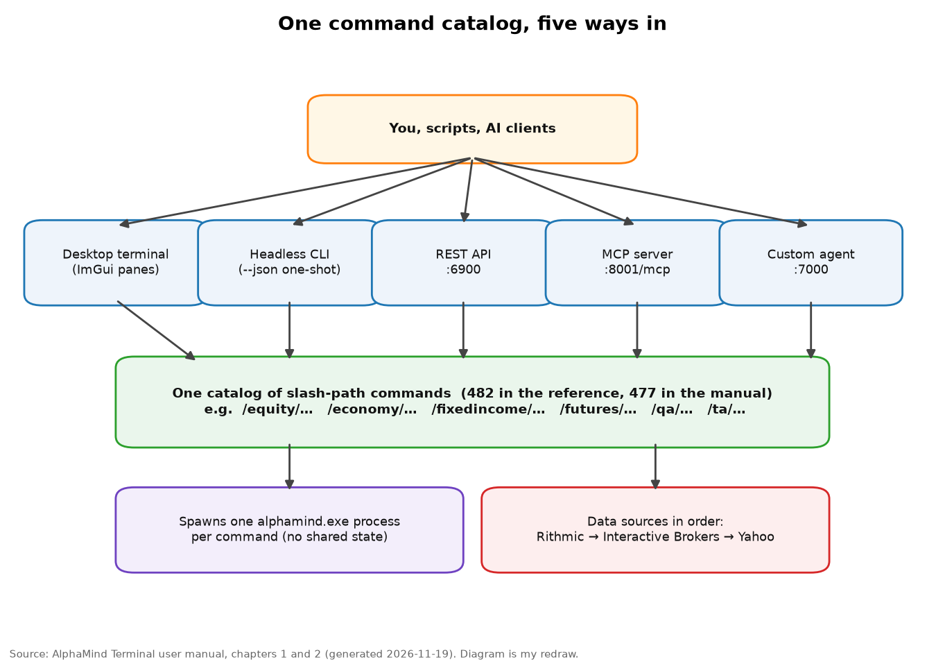
The architecture is deliberately simple. The REST API, the MCP server and the agent all live in one folder of Python code. Each command run spawns one process of the executable, so the Python layers are thin wrappers around the same compiled program the desktop uses. The agent talks to the MCP server, the MCP server talks to the executable, and a language model, hosted or local, sits on top.
There is a design choice buried in that one-process-per-command rule that has consequences throughout the platform, good and bad. The good: a command that crashes or hangs cannot take the terminal down with it, and the web-facing layers never run your analysis inside their own memory. The bad: nothing is remembered between commands. The quantitative and technical-analysis commands keep their state only inside one process, so a command line call that loads a price series and a second call that computes a drawdown will not find each other. The documentation is blunt about this. It tells you to load and analyze in a single call, using a pipeline.
Why “every menu item is a command” matters
The manual states a rule that is easy to read past: every menu action runs a slash command, so anything you can click you can also type, script or call over REST and MCP. The consequence is that there is no hidden functionality in the graphical interface. A feature either exists in the catalog, in which case a script and an AI agent can use it, or it does not exist.
For AI agents this is the crucial property. Agent frameworks fail most often not because the model is weak but because the tools it was handed do not cover what the human sees on screen. Here the screen and the toolbox are the same object. When you ask the agent to “show the macro overview,” it runs the same command that the Economy menu runs, and you can reproduce the answer by typing it yourself.
The command syntax in one paragraph
Commands are slash paths in the style of a file system. Arguments are space-separated positional strings, and the parser has no quoting, so multi-word values must be split into separate arguments or replaced with single-word categories. Optional arguments are shown with their defaults in the usage string. Data commands built on Yahoo accept a source flag that forces one of three data sources. The default priority is the futures data network first, Interactive Brokers second, and Yahoo third, and the order is itself a setting. If you force a source that lacks a capability, the command says so rather than falling back silently, with a message of the form “not supported by” that source.
Every result has the same shape: the command that ran, an overall OK flag, a list of log lines tagged with a level such as info or error, and an optional table with a title, a list of columns and a list of rows. Over the command line the exit code is zero for success and one for an error, a timeout or an unknown command. The reference repeats a rule that I wish every data tool printed on its first page: never treat a missing table as data, and report the error text. We will see why in a later section.
The catalog: 482 commands in 29 modules
The programmer reference’s contents page is the best map of the platform. Here is the whole catalog, sorted by size.
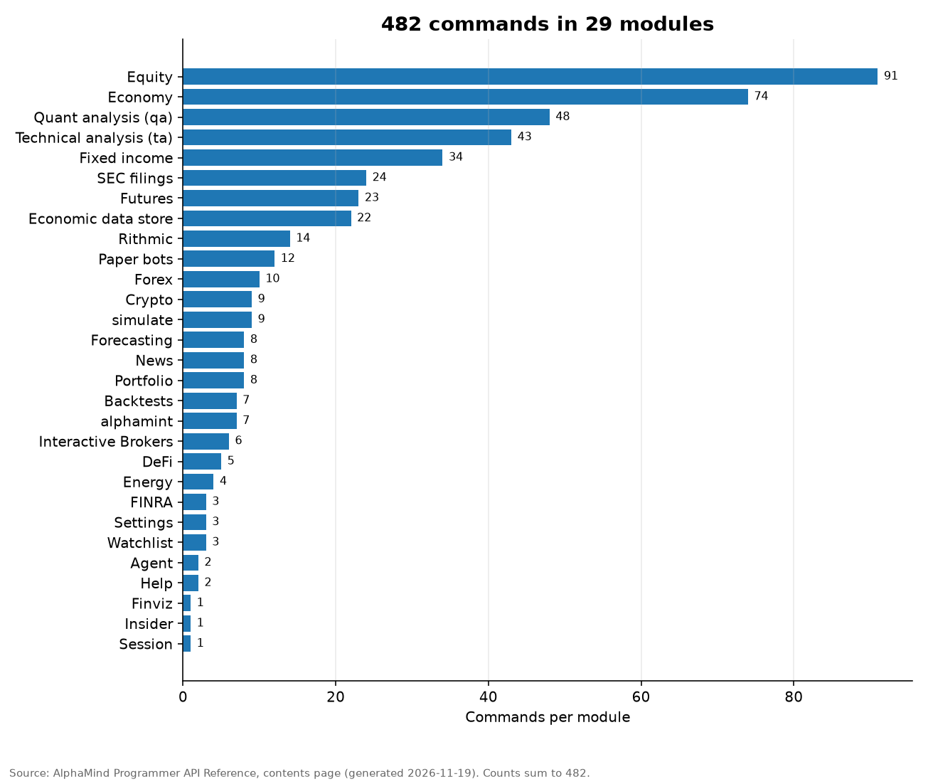
Three things stand out. First, the catalog is broad but not random. The three largest modules, equity at 91 commands, economy at 74 and quantitative analysis at 48, are the ones a research desk uses daily. Technical analysis is next at 43 and fixed income follows at 34. Together those five account for 290 of the 482 commands, which is just over 60 percent of the platform.
Second, the catalog treats government and regulatory data as first-class. There are 24 commands for SEC filings, covering full-text search of EDGAR, XBRL company facts, parsed insider transactions from Form 4, 13F institutional holdings, fund portfolios from N-PORT filings, and the adviser-registration database. There is a separate three-command FINRA module for short interest and off-exchange volume, and a one-command module for insider trades. The economy module is not a single FRED wrapper either. It reaches the BLS for payrolls, CPI, PPI, job openings and demographics, the New York Fed for reference rates, reverse repo operations and the Fed’s securities portfolio, the CBOE for volatility indexes and put-call ratios, the IMF and OECD for cross-country indicators, USAspending for federal contracts, a shipping-chokepoint tracker, and the Ken French factor library.
Third, the catalog is honest about layers. The futures module has 23 commands and the Rithmic module has 14, and they split cleanly: Rithmic is the data connection and contract-metadata layer, while the futures module holds the analytics, such as cost of carry, basis, roll yield, curve classification, Black-76 option pricing, implied volatility, spread payoffs and hedge sizing. Many of the futures analytics are explicitly marked offline, which means they work from numbers you supply and need no live feed.
What “offline” buys you
Whenever I read a list of financial calculators, I look for the ones that need no data connection. Those are the ones you can trust in a classroom, a code review, or an agent loop that must not wander off to a flaky network source. The reference marks several: bond pricing with duration, convexity and DV01 from a coupon and a yield; yield to maturity from a quoted price; a Nelson-Siegel-Svensson curve evaluator; mortgage payment and amortization schedules; an implementation of the CME FedWatch probability arithmetic from a futures price; Black-76 option pricing and Greeks from explicit inputs; and a multi-leg option-spread tool that returns net premium, maximum profit and loss, breakevens and net Greeks. In a few sections we will use their math as a vehicle for explaining the concepts behind them.
The desktop terminal
The desktop is an ImGui application, which means a dense, dockable, keyboard-friendly interface in the tradition of terminal software. The menu bar has File, View, Equity, Economy, Crypto, News, Watchlist, Bot, Alerts and Help. Panes include a watchlist, a chart, a command pane, an agent chat, an alerts monitor and logs, and each pane can be minimized, maximized or closed.
The command pane works the way a shell does. Tab completes a command path, Enter runs it, and the up and down arrows walk your history. Results appear as tables in the pane and as log lines. The Help menu runs a command that lists every command, which is also how the manual’s complete reference was produced.
One screenshot in the manual shows the Bot pane, which I will discuss in detail later. I have blanked out two folder-path fields and the example values in the bottom form, so that no local directory names or sample bot parameters appear here.
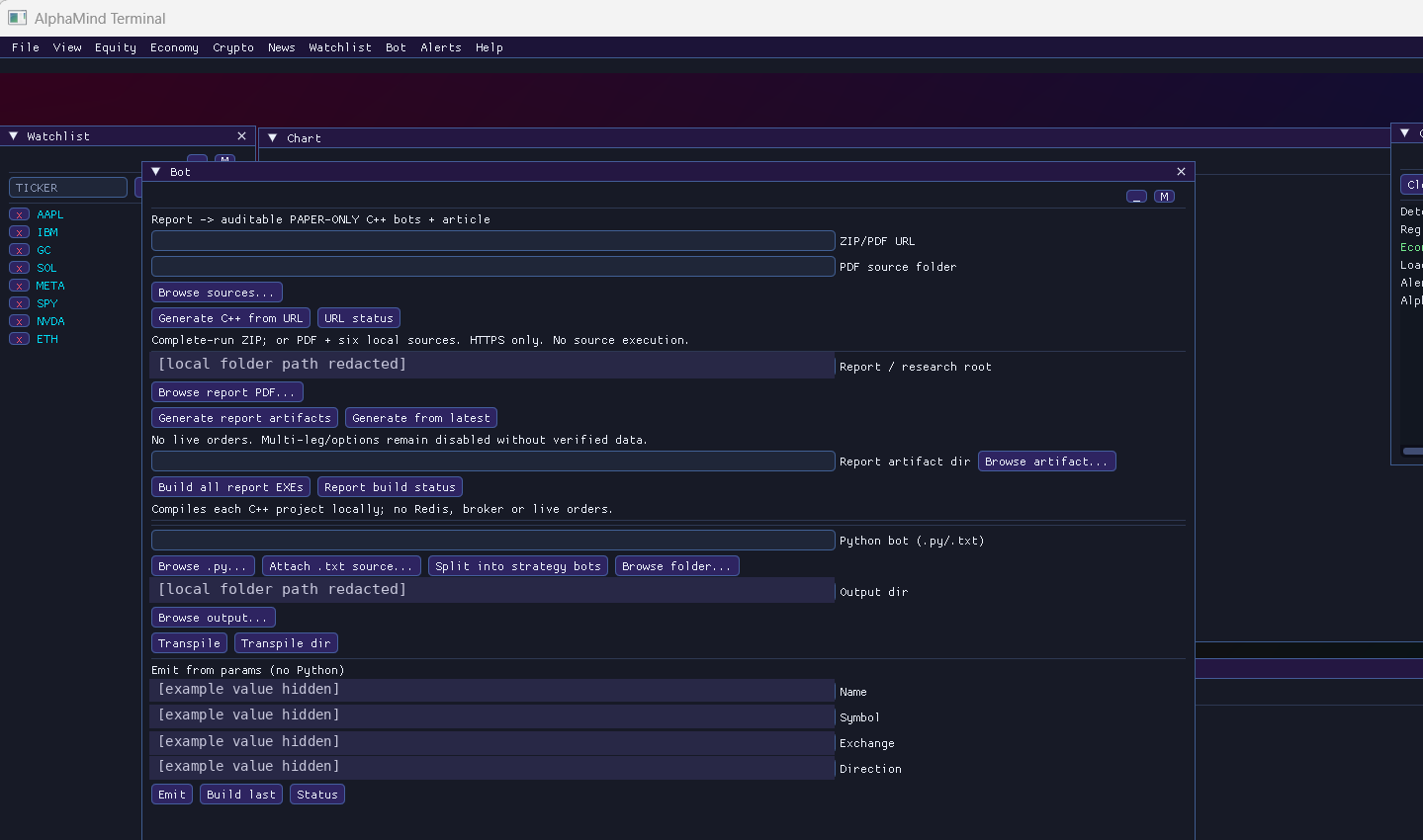
Even in this one image you can see the platform’s design philosophy. The Bot pane is a research-to-paper-bot generator: its labels describe turning a research report into “auditable paper-only” C++ bots and an article. Underneath the form fields, the text states in plain words that it makes no live orders, that multi-leg and options strategies stay disabled without verified data, and that the generated projects compile locally with no Redis, no broker connection and no live orders. A tool that tells you what it will not do on the face of its own interface is rare, and it is a good sign for anyone planning to put an AI agent near it.
The alert monitor
The alerts menu deserves a mention because it is where the AI layer meets the news. The monitor polls a news API for keywords and symbols you configure, can optionally ask the configured model to score the urgency of each item, and can automatically trigger an agent analysis when a story’s urgency reaches a threshold you set. The manual notes a practical limit: on the free news plan you should keep the polling interval at 60 seconds or more. It is a small feature, but it shows the pattern the platform wants to follow: deterministic commands do the fetching and arithmetic, and the model is used for judgment on top.
The REST API: any program, no SDK required
The REST layer is a small Python service. The manual documents a handful of endpoints: a health check that reports status, the executable path and the command count; a command catalog, optionally filtered by family; a route per command, called with a POST to a path that starts with the version prefix and continues with the command’s own slash path; a pipeline endpoint that runs several commands in order; and an administrative reload. A few extra endpoints describe the platform to a Workspace as widgets, apps and agents.
The request body is a small JSON object with a list of arguments, an optional source, a confirm flag that is false by default, and a timeout. The response is the same result object described earlier, plus the exit code. If you can make an HTTP request from your language of choice, you can use the entire catalog. The programmer reference goes further and gives, for every one of the 482 commands, a Python example using a bundled client library, a Python example that spawns the command line and parses JSON, a C++ example using a bundled header, a C++ example that spawns the executable, and the MCP tool call. That is five ways to call 482 commands, documented, which is why the reference is nearly 500 pages long.
Errors that mean something
The REST error table is short and precise. A 401 means a missing or invalid API key. A 403 means orders are disabled on the server, by design. A 404 means an unknown command or route. A 422 means an invalid body or control characters in an argument. A 5xx or 504 means the process failed or timed out. The troubleshooting chapter adds the human version of these: a 422 with a JSON decode error almost always means that shell quoting broke the body, and the fix is to send the body from a file.
I would have liked to see all of this earlier in my own career. A trading research API that distinguishes “you were not allowed to place that order” from “that route does not exist” from “your JSON was malformed” saves hours of confusion, and it also gives an AI agent clear signals to reason about.
Security defaults
The manual’s security section is short and the posture is sensible. The service binds to the loopback address by default. If you set an API key, protected calls require it in a header. Arguments reach the underlying process as an argument list rather than through a shell, and only registered command paths exist as routes. Cross-origin access is limited to localhost and a Workspace. The checklist at the end of the manual adds that keys live only in the configuration file or in environment variables, never in documents or chat, that any key ever pasted into a shared place should be rotated, and that before binding to anything other than loopback you should set the API key and the MCP token and put TLS in front.
Notice what is not claimed. The documents do not say the platform is hardened for the public internet, and they tell you not to expose it without extra steps. I mention this because “AI agents with API access to a trading platform” is exactly the sentence that should make a careful reader ask what happens when it is exposed. The documents answer with defaults that keep it local.
Starting the whole stack
The start order is documented as a four-step table: first the data services, which are Redis and the futures gateway and are needed only for live futures prices; then the REST API; then the MCP server; then the agent. Each service is a plain process and you stop them in reverse order. The REST API is independent of the rest.
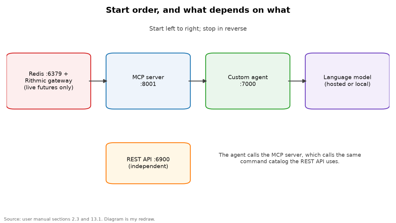
The manual is clear that offline commands, including equity, economy, crypto, futures math and Rithmic metadata, need none of the live infrastructure. That is a big practical point. A user can install the terminal, never connect a broker or a futures gateway, and still use hundreds of commands.
Pipelines: how analysis survives a stateless process
Earlier I described the stateless rule. Here is why it is the single most important thing to understand about the platform if you plan to use an AI agent with it.
Quantitative commands work on a dataset that you load first. The command to load a ticker’s data into the analysis session is separate from the commands that compute returns, risk or drawdown. Technical-analysis commands work the same way: you load a symbol, add indicators to a chart, and list or remove them. But because each command in the command line or REST interface runs in a fresh process, the loaded data would be gone by the time the next command started.
The solution is the pipeline: an ordered list of commands executed inside a single request. The MCP server’s version of it chains up to 20 steps, stops at the first failure, and lets later steps reference earlier results. In pseudocode, a risk analysis looks like this.
pipeline = [ load(ticker), returns(), value_at_risk(confidence), expected_shortfall(confidence), max_drawdown() ]
result = run_pipeline(pipeline)
if any step failed: report the error text and stop
else: summarize the tables returned by each step
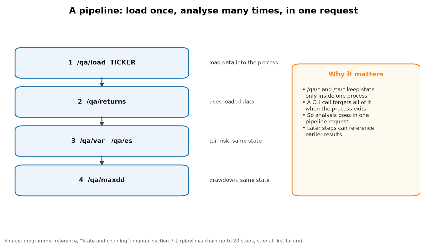
I like this design for two reasons. It makes agent behavior auditable, because the whole analysis is a single declared object rather than a sequence of invisible side effects. And it makes analysis reproducible: you can store the pipeline, run it again tomorrow against fresh data, and compare. A pipeline is also a natural unit to hand to a human reviewer. It reads like a short recipe.
The MCP server: the catalog as AI tools
The Model Context Protocol is a standard way for AI clients to discover and call tools. The platform’s MCP server presents the command catalog as MCP tools using FastMCP, and it supports three transports: streamable HTTP, server-sent events, and standard input and output for clients that launch the server themselves. The manual gives configuration snippets for VS Code and for a Claude Desktop style client.
What interests me is not that the platform has an MCP server. Many tools do. It is how the server decides what to expose. There are three levels, chosen at startup. The smallest, called meta, exposes four tools only. The default, called core, adds a curated set of named commands, including those for the bot libraries. The largest, called all, exposes one tool per command.
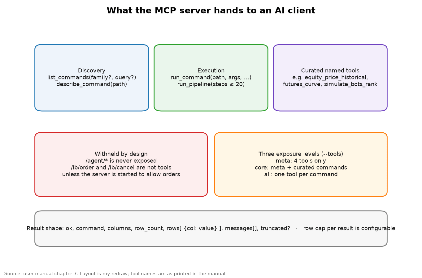
The four meta tools are the clever part. Two of them handle discovery: one lists commands, optionally filtered by family or a search phrase, and the other describes a single command, returning its usage text. The other two handle execution: one runs any allowed command with arguments, an optional source, a timeout and a row cap, and the other runs a pipeline. With only those four tools an agent can find any command in a 482-command catalog, read how to call it, call it, and chain calls together. It does not need 482 tool definitions stuffed into its context window. That is a pragmatic answer to a real problem: tool lists that grow past what a model can use well.
The curated tools such as historical equity prices, the futures curve, and the listing, ranking and validation of the bot libraries give the model clear, named handles for the most common jobs. Result rows are capped, with a default of 200 rows per result, and the results carry a flag saying whether truncation occurred. A model that is told its answer was truncated can ask for a narrower query instead of silently reasoning about incomplete data.
What the server will not expose
Two exclusions are written into the manual. The agent command group is never exposed through MCP, which prevents an agent from calling another agent in a loop through the tool interface. And the order and cancel commands are not tools unless the server was started with an explicit flag that allows orders. Even then, the one order tool is documented as a dry run unless a confirm argument is set to true. Remote access requires a bearer token.
The manual is also open about what it has not tested. The server-sent-events transport has not been exercised with a real third-party client on the documented installation, although the standard-input and streamable HTTP transports are covered by the test suite. I will quote the manual’s “did not verify” list in full later, because I think every product document should have one.
The custom agent: plain-language questions, bounded tool loops
The built-in agent is a small service that answers plain-language questions by calling MCP tools through a language model. You can use it in three ways: a one-shot question on the command line, an HTTP server with a web chat page, or a mode that starts its own MCP server and talks to it over standard input and output. The manual’s own example question is “Rank the simulate bots by sharpe, top 5,” and another is simply “What is the macro overview?”
The agent’s HTTP interface is more complete than I expected. There is a status endpoint that reports whether the MCP server is reachable, which provider and model are configured and whether a key exists, but never the key itself. There are endpoints for the available models, for the tools visible to the model, for a streaming query that emits server-sent events of types status, tool call, tool result, message and done or error, and for a non-streaming chat call that returns the final answer along with the full trace of tool calls. The streaming interface is how a user interface can show the agent’s work as it happens. The trace is how a reviewer can check it afterward.
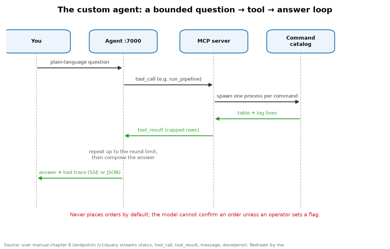
In pseudocode the loop is straightforward.
history = [ system_rules, user_question ]
for round in 1 .. max_rounds:
reply = model(history, tools = visible_tools)
if reply has no tool calls: return reply.text plus the full tool trace
for each tool call: run it through the MCP server, append the capped result to history
return the best answer so far, noting that the round limit was reached
Which models
By default, when a hosted-model key is configured, the desktop Agent pane, the agent service and the AI features inside the sub-projects all use a hosted multi-model service, and no other setting is needed. The manual lists a curated set spanning several families: Claude, GPT, Gemini, Grok, and open-weight models such as Llama, DeepSeek, Mistral and Qwen. It notes that the live model list comes from the agent’s models endpoint, that the curated list is only a fallback, and that availability depends on your account. I am not going to repeat the individual model names, because they will age quickly, and the document itself tells you to read the live list.
For people who want everything on their own hardware, the manual describes a local-model path: set the provider to local, give it the base URL of an OpenAI-compatible server such as llama.cpp’s server or Ollama, and choose a model that supports function calling. It includes a warning that anyone who has run local models will recognize: a model without function calling will answer in text and never call a tool, and the fix is to start the server with a tool-aware chat template or pick a different model.
Guard rails on the model itself
The agent’s behavior is bounded in several documented ways. It has a maximum number of tool rounds per question, with a default of eight in the agent service. Its system prompt carries rules for working with the bot libraries, and the manual states the house rule for data plainly: never fabricate data, and when a command returns no data or an error, report it as it is. Its HTTP interface can be protected with its own key. And, crucially, the model cannot place orders by default, and cannot even pass the confirm argument unless an operator sets a specific environment flag.
I want to dwell on that last point, because it is the difference between an AI demo and an AI system you could imagine pointing at real work. The agent is not asked to be careful. The server is built so that the careless path does not exist. The next section looks at the order-safety design more closely.
Order safety: independent gates on every path
If you are going to let an AI agent near a trading platform, the first question is not how smart the agent is. It is how many separate things have to go wrong before it can send an order. The manual’s answer, scattered across several chapters, is that there is exactly one order path in the whole catalog, and that it is guarded by independent gates at every layer.
The one path is a command for placing an order with Interactive Brokers. Here is what stands between a request and a live order, according to the manual.
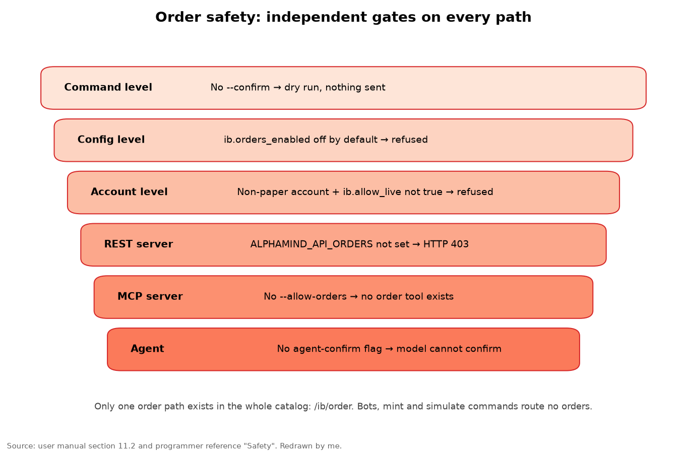
At the command level, an order without the explicit confirm flag is a dry run and nothing is sent. At the configuration level, orders are refused unless a setting named for enabling orders has been turned on, and it is off by default. At the account level, an order on a non-paper account is refused unless a separate allow-live setting is true. At the REST level, the route returns a 403 unless the server’s operator set an environment variable allowing orders. At the MCP level, there is no order tool at all unless the server was started with the allow-orders flag. At the agent level, the model cannot pass the confirm argument unless an operator sets one more flag.
These are layers in the sense of the old “Swiss cheese” model of safety. Each layer has holes, but the holes are in different places. If we call the probability that layer i fails open in a given session pᵢ, and the failures are independent, the chance that an unintended order gets through is the product of those probabilities. The point is not the numbers, which the documents do not give and I will not invent. The point is that independence turns a sum of risks into a product, and a product of several small numbers is very small. Where layers are not independent, for example if one operator flips every switch at once, the protection collapses, and that is a human process problem the documents rightly leave to the checklist: leave the orders-enabled setting off unless you intend to trade.
Paper by construction
Everything under the bot, alphamint and simulate command groups is described as paper or research only, and the manual says that nothing under those groups routes orders. This is a stronger statement than “we do not place orders by default.” It says the order code simply is not reachable from them. The developer chapter reinforces it with an instruction that I wish more codebases carried: when adding a new command, keep it read-only unless it is an explicit, gated action, and never add a second order path.
I would like to be careful about what this does and does not tell you. It tells you how the platform is designed. It does not tell you how any particular installation is configured, and the manual explicitly lists interactive-broker connectivity and running bots among the things it did not verify. A design is a promise; a deployment is a fact. The honest summary is that the design is cautious in the right places.
A note before the paywall
I split this article in two on purpose. Everything above is the platform overview that anyone should be able to read: what the two documents are, how the five interfaces fit together, how the MCP server and the agent work, and how order safety is designed. Everything below is the deeper tour for paid subscribers: the data sources, an honest look at what the reference’s own sample outputs show, and then the quantitative, technical, fundamental, fixed-income, futures and portfolio toolkits with the math behind them, a section on backtesting and bot research that I am keeping conceptual, and my ideas for where this could go.
Two things you do not need a subscription for. First, the PDFs. If you want the 60-page user manual and the 487-page programmer reference, send me a Substack direct message or an email asking for them, and I will email them to you as soon as I can. Second, a conversation. If you want to learn more about what is offered, or you have an idea for what you would build on a platform like this, message me. I read everything, and the best ideas in this space are going to come from people who use these tools, not from the people who write the documentation.
And the question I promised: where do you think this goes, and what would you like to do with it? Would you point an agent at it to produce a morning research brief? Run a risk review on a portfolio? Audit a trading idea before it gets near a broker? Teach a class? Tell me in a comment or in a message, and I will build the next article around the answers.
Data: a priority list, plus a long tail of public sources
Every research platform lives or dies on its data. This one takes an unusual approach: it does not try to be a single vendor. It has a priority list of three primary sources for prices and a very long tail of public and keyless sources for everything else.
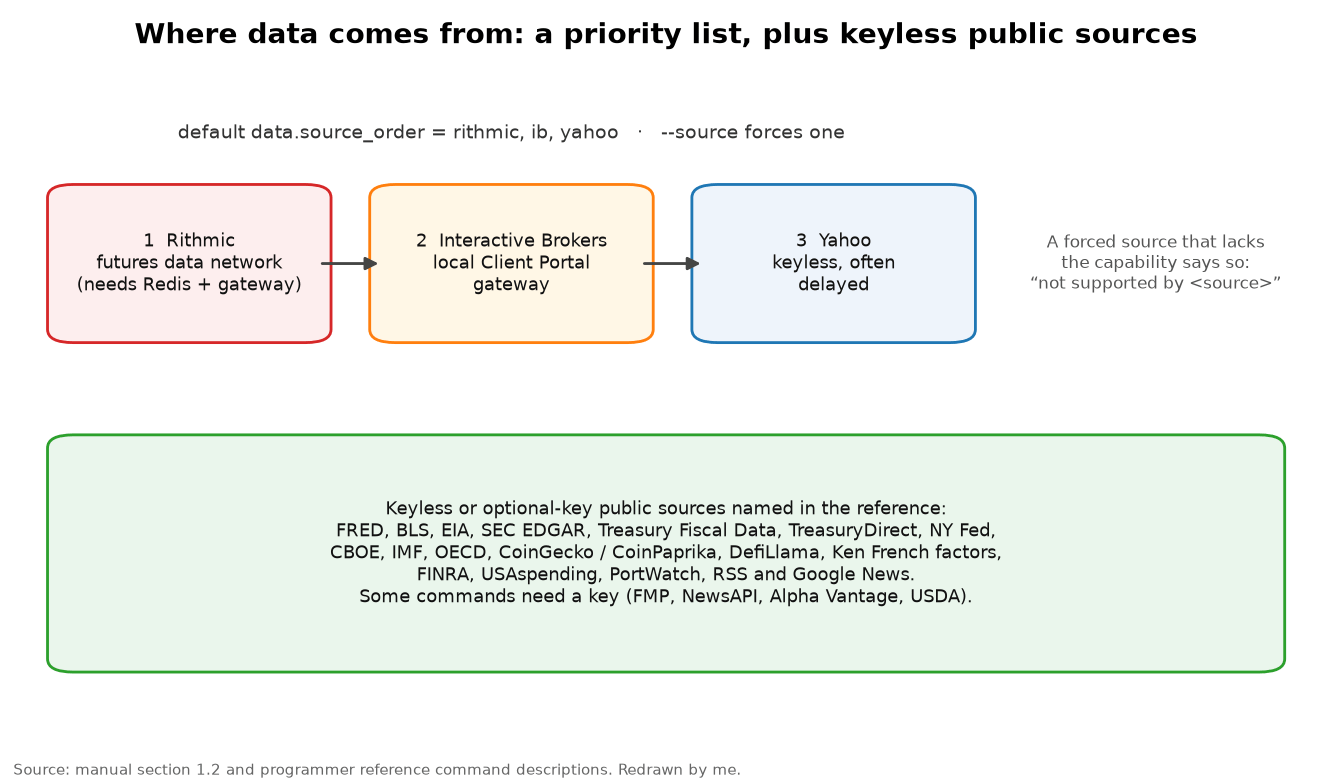
For prices, the default order is the futures data network, then the Interactive Brokers gateway, then Yahoo. Live futures need Redis and the futures gateway running, while Yahoo is keyless and can be delayed. The order is a setting, and any call can override it. The design question that always follows is what happens on disagreement. The documents’ answer is not reconciliation but transparency: each command says what it used, and a forced source that does not support a capability returns an explicit message.
For everything else the reference leans on public data. Macro series come from FRED with an optional key and a free fallback that needs no key. Labor, inflation and job-openings data come from the BLS. Energy comes from the EIA. Filings come from SEC EDGAR. Treasury yields, auctions, debt and budget data come from Treasury sources. Volatility indexes and put-call ratios come from the CBOE. Cross-country data come from the IMF and OECD. Crypto prices come from CoinGecko and CoinPaprika, and DeFi data come from DefiLlama. Some commands need a key for a commercial provider, and the descriptions say so, for example “needs key” for a fundamentals endpoint that has a free alternative.
The manual states the key-handling rule in one line: keys live only in the configuration file or in environment variables, never in documents, chat or version control. The desktop’s agent pane shows whether a key is configured but never displays it, and the agent’s status endpoint does the same. I checked both documents for anything that looked like a credential, and the only thing resembling one is the manual’s status capture of the futures connection, which prints masked values with asterisks. That is the right way to show a status screen in a document you plan to share, and I will not reproduce even the masked values here.
Reading the sample outputs critically
This section is the one I most want you to read, because it is where I think the platform’s documentation is at its best, and also where it shows exactly what an AI agent using the platform would need to be careful about.
The programmer reference runs a sample call for every one of its 482 commands, using placeholder arguments, and records what happened. I tallied the outcomes.
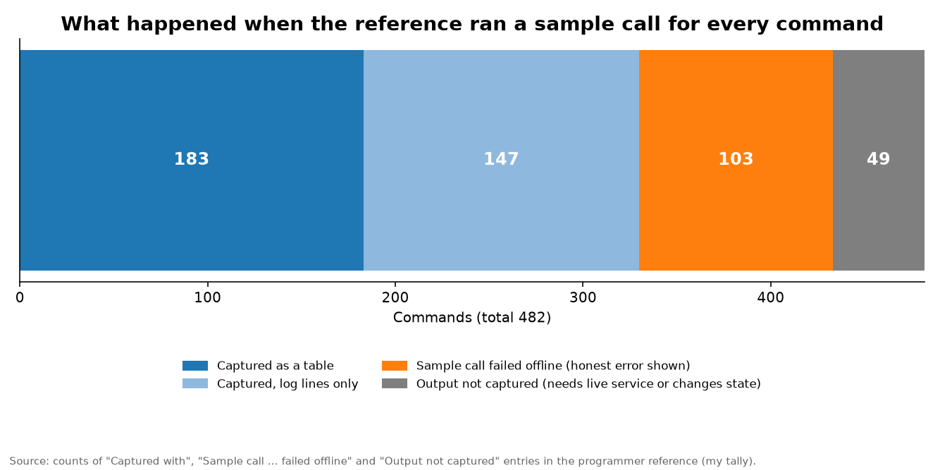
Of 482 commands, 330 have a captured result: 183 returned a table, and 147 ran successfully but produced only log lines. Another 103 sample calls failed in the offline environment where the reference was generated, and the reference prints the error as it happened. The remaining 49 are marked as not captured because they need a live service, credentials, or change state. The 330, 103 and 49 add up to 482, which is the kind of arithmetic I like to see work.
The failures are instructive and, to my eye, reassuring. A sector-rotation backtest sample fails with a message that you need at least two comma-separated symbols. A crypto sample fails with an HTTP 404 from a data provider because the placeholder coin does not exist. A FRED sample fails with a 400 because the placeholder series does not exist. A government-data sample says that no key is configured and tells you where to register for a free one. A pipeline sample says it could not open a temporary output file. None of these are bugs in the interesting sense. They are the platform telling the truth about a bad input, which is precisely what you want from the tool layer under an AI agent.
What the manual admits it did not verify
The manual closes with a short section titled “What this manual did not verify.” It lists four things: calls to the hosted model service and its live model list; Interactive Brokers, futures-gateway and Redis connectivity along with running bots; the server-sent-events MCP transport with a third-party client, a Workspace and the VS Code MCP integration; and the C++ REST example. The earlier part of the manual adds that running the bots live needs Redis, the futures gateway and the bot dependencies, none of which were exercised for the manual.
Another honest detail: the manual deliberately includes a sample of a failing command. Its crypto example shows an “unknown command” error for a command path that the manual’s own catalog does not contain, with exit code 1 and the message suggesting you try the help command. The manual uses it to show the error path. It is a small thing, but a document that prints its own failure modes is a document that can be trusted to print the rest.
The documents also disagree with each other by five commands, 477 against 482. The difference is the five pipeline commands in the simulation module: the reference lists nine commands there and the manual’s table lists four. A reader who only saw one number would not know. A reader who saw both can ask which document is newer, and that is the sort of question the PDFs make easy to ask.
What the samples teach about validating an AI agent’s inputs
Later in this article I will show a few places where the printed samples look surprising: a buy-and-hold backtest on one of the largest stocks in the world that prints a total return of exactly minus 100 percent and forecasts that sit far below the quote printed in the same capture. I raise this early because it changes how you should think about agents and platforms like this one. The platform’s job is to produce outputs. An agent’s job is to use them. Neither, on their own, check that the outputs make sense. The most valuable thing a research agent can do may be to run sanity checks, such as comparing a buy-and-hold result with the ratio of the first and last price, before it writes a single sentence of analysis. I will return to that idea when we get to backtesting.
The quantitative toolkit: returns, risk, and the ratios everyone argues about
The quantitative-analysis module has 48 commands, and the complementary econometrics module has 22 more. Both work on a loaded dataset. They cover descriptive statistics and rolling windows; returns, differences and cumulative sums; volatility, variance and standard deviation; skewness, kurtosis and quantiles; the standard performance ratios; tail-risk measures; drawdown; normality and unit-root tests; autocorrelation; change-point detection; seasonal decomposition; and the capital asset pricing model. The portfolio module adds a single command that returns a full risk and performance scorecard, including the Sortino and Omega ratios, the Calmar ratio, conditional value at risk and the ulcer index.
I will use this section to explain the math that those commands correspond to, because it is the part of the platform that is most useful to a student and the part where an AI agent most needs to be fed correct definitions. Everything in the equations below is standard textbook material. The reference describes each command in a single line and does not print its implementation formula, so treat these as the definitions the commands are named for, not as a statement about the exact code.
Returns and the Sharpe ratio
Quantitative work starts with returns. The convenient version for analysis is the log return, because it adds across time.
The Sharpe ratio scales an average excess return by its volatility, and annualizes by the square root of the number of periods per year, 252 for daily data.
The Sortino ratio changes only the denominator. Instead of penalizing all volatility, it penalizes only the downside, using the root mean square of returns below a target.
The Omega ratio goes a step further and looks at the whole distribution. It is the expected gain above a threshold divided by the expected shortfall below it, so it reflects skewness and fat tails that a mean and a standard deviation cannot see.
Why print three ratios? Because they disagree, and the disagreement is information. A return stream with a smooth upward drift and a rare crash will score well on Sharpe and poorly on Sortino and Omega. A stream with frequent small losses and occasional big gains will look the opposite. A platform that reports all three side by side, in one command, nudges the user toward looking at the shape of the distribution instead of at one flattering number.
Value at risk and expected shortfall
Value at risk asks a simple question: what loss will be exceeded on only one day in twenty, if α is 95 percent? It is a quantile of the return distribution. Under a normal-distribution assumption it has a closed form in the mean, the volatility and the matching normal quantile.
Expected shortfall, also called conditional value at risk, answers the follow-up question: when the bad day arrives, how bad is it on average? It is the mean of the returns beyond the value-at-risk line, and for a normal distribution it also has a closed form that involves the normal density.
The reference prints a real example I can use to show both ideas. Its sample risk-and-return capture for a large technology stock reports an annualized return of 21.78 percent, an annualized volatility of 28.14 percent, a 95 percent daily value at risk of minus 2.72 percent, a skewness of 0.40 and a kurtosis of 6.54 on 1,252 observations. Those are the platform’s printed values; I have not verified them against a data vendor.
I can check one thing, which is whether the printed value at risk is consistent with the printed volatility. Dividing the annual volatility by the square root of 252 gives a daily volatility of about 1.77 percent. The daily mean is about 0.09 percent. Plugging both into the normal formula with the 95 percent quantile of minus 1.645 gives a normal-theory value at risk of about 2.83 percent. The printed historical figure of 2.72 percent is slightly smaller. For a distribution with a kurtosis well above three, that is not surprising: fat-tailed distributions concentrate more of their probability near the center and in the extreme tails, which can push the 95 percent quantile in a little while pushing the 99 percent quantile far out. The reference does not say whether its kurtosis is raw or excess, so I will not lean on the exact figure, but a value of 6.54 under the raw convention would still be more than twice the normal value.
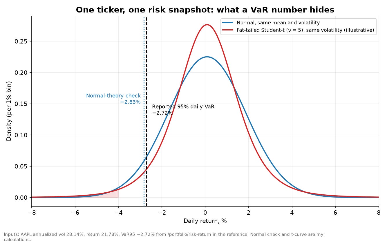
In the figure, the blue curve is a normal distribution with the printed volatility and mean. The red curve is a fat-tailed Student-t distribution with the same volatility, which I chose purely for illustration. The two vertical lines are the printed value at risk and my normal-theory check, and they are nearly on top of each other. That closeness is the trap. Value at risk at 95 percent is nearly blind to the difference between the two curves. The shaded region far in the left tail is where they differ, and that is the region expected shortfall is designed to look at. If a platform gives you both numbers in one pipeline, you can see the tail instead of just a single cut-off point.
Beta, alpha and the factor world
The platform’s capital asset pricing command and its portfolio performance command are built on the same regression. An asset’s excess return is regressed on the market’s excess return. The intercept is Jensen’s alpha, the slope is beta, and the residual is everything the market does not explain.
The platform also ships the Ken French factor library, with the three-factor, five-factor and momentum datasets available as commands. A factor dataset next to a regression command is more powerful than it looks. It means a user, or an agent, can go from “what is this stock’s beta?” to “how much of this strategy’s return is explained by size, value, profitability, investment and momentum?” without leaving the terminal. I will not claim the reference demonstrates that workflow end to end, because its sample captures show only the first two rows of each table. But the pieces are there.
The econometrics module
The econometrics group is a small statistical workbench: a data store where you can load, index, type, transform and export datasets; ordinary least squares and panel regressions with a comparison command; diagnostic tests for serial correlation and heteroskedasticity; and tests for correlation, normality, unit roots, cointegration and Granger causality. Most of the sample captures for these commands show only log lines because they operate on a dataset the sample call did not load, which is a consequence of the stateless design rather than a defect.
For a research agent, the interesting ones are the tests that stop you from fooling yourself. Cointegration protects you from spurious regressions between trending series. A unit-root test tells you whether you are about to model a price level as if it were stationary. Granger causality tells you whether one series helps predict another beyond that series’ own history, which is a much more modest claim than the word “causality” suggests.
Time series and forecasting: what a baseline is for
The forecasting module has eight commands: autocorrelation with a significance band, a seasonal decomposition, and six baseline forecasters. The documents are open about what they are. The descriptions say things like “baseline forecast” and “pure C++ baseline.” The forecasters are a linear trend fitted by ordinary least squares, Holt’s double exponential smoothing, an additive Holt-Winters command that reduces to Holt when its seasonality setting is zero, a random walk with drift, an autoregression on differenced data fitted by least squares with no moving-average term, and the standard theta method, described as simple exponential smoothing plus half of a linear drift. Their documented default fit window is 1,260 days, roughly five years of trading days. They return a table of steps, dates, point forecasts and 95 percent intervals.
Autocorrelation and the trap of price levels
The autocorrelation function measures how strongly a series correlates with its own past at each lag, and the reference’s significance column tests each lag against what white noise would produce. For a sample of n observations, an autocorrelation outside roughly plus or minus 1.96 divided by the square root of n is flagged.
The reference’s sample capture shows the autocorrelation at lag one for a stock price series as about 0.975, flagged significant. With roughly 1,254 observations, which I infer from the row count of the decomposition sample, the band is about plus or minus 0.055. A value of 0.975 is so far outside that band that the test is nearly meaningless, and that is exactly the point. Price levels are close to a random walk, and a random walk has an autocorrelation function that decays very slowly. Applying a white-noise test to a price level is asking the wrong question. You want it on returns.
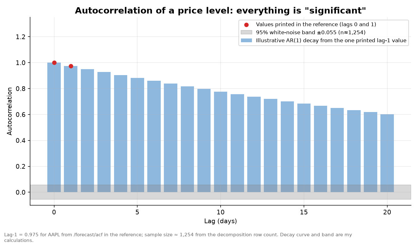
I drew an illustrative decay curve from the one printed value, assuming a simple first-order autoregression, to show what such a series looks like against the band. Only lags zero and one are printed in the reference, so the other bars are my illustration and not output from the platform. The practical lesson for anyone building an agent on top of this: tell the agent which series to test, and why. The tool will happily answer whichever question you ask.
The same reasoning is behind the unit-root commands. The augmented Dickey-Fuller test fits a regression of the change in a series on its lagged level and lagged changes, and tests whether the coefficient on the lagged level is zero. If it is, the series has a unit root and behaves like a random walk. The platform pairs it with a KPSS test, whose null hypothesis is the opposite one, so you can check whether the two agree.
Change points
A related command detects change points with a CUSUM statistic. The idea is old and elegant. You accumulate deviations from a reference mean, subtract an allowance so that small noise does not accumulate, and floor the sum at zero so that old good news cannot cancel new bad news. When the accumulated sum crosses a threshold, you flag a change.
For a strategy review this is a useful tool: it asks whether a stream of results has drifted away from the level you thought you were getting. I am deliberately keeping this general. The thresholds and allowances you would choose for any particular case are your own business, and the point here is the concept.
Baseline forecasters
Holt’s method keeps a level and a trend, and updates both with exponential smoothing. The h-step-ahead forecast is the level plus h times the trend.
Now look at what the reference prints for the first two forecast steps of three of its baselines on the same stock, all in the same capture where the last quote is 349.21.
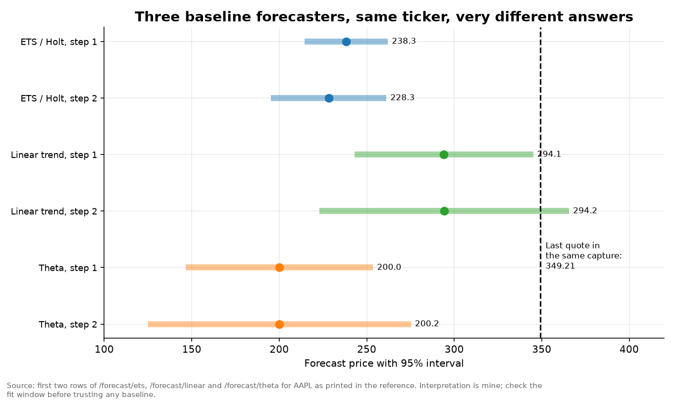
The exponential-smoothing forecast is about 238 for step one with a 95 percent interval from about 216 to 260. The linear-trend forecast is about 294, with an interval from about 245 to 343. The theta forecast is about 200, with an interval from about 148 to 252. All three sit below the printed quote, and they disagree with one another by nearly 100 dollars on a stock trading around 349. If these were predictions, that would be alarming. As baselines they are doing their job in an unexpected way, by showing that the answer depends heavily on the method, and that a user should not read any one of them as a forecast of price. Their usage lines show the same default fit window of 1,260 days, so the gap comes from the methods rather than from different data, and I would want to understand that before trusting any of them.
There is one thing that does check out beautifully. For each of the three baselines, the width of the 95 percent interval at step two is almost exactly 1.414 times its width at step one. That is the square root of two, which is what you expect when forecast uncertainty grows with the square root of the horizon, as it does for a random walk with independent shocks. I computed the ratios myself from the printed values: 62.5 divided by 44.2 for the smoothing model, 139.4 divided by 98.6 for the linear model, and 146.7 divided by 103.8 for the theta model, all equal to 1.414 to three decimals. The platform’s interval arithmetic is internally consistent even though the point forecasts are puzzling.
Two more notes from the same table. The exponential-smoothing and Holt samples print identical first rows, which is exactly what the reference’s own description predicts, since the first is the second with seasonality switched off. And the autoregression and random-walk-with-drift samples print values like minus 6.6 and minus 0.13, which are not price levels. The autoregression is documented as working on differenced data, so those rows are probably changes rather than prices, but the result table does not say so. When an agent reads this table, it needs to know the scale of the column. A one-line “units” field in each result would be a cheap and valuable addition.
Technical analysis: 43 commands, and what they have in common
The technical-analysis module has 43 commands. I grouped them by job, which is my own organization and not the reference’s, because a long alphabetical list hides the structure.
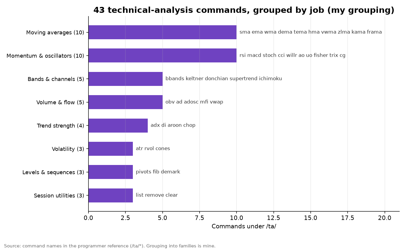
Ten are moving averages in different flavors: simple, exponential, weighted, double and triple exponential, Hull, volume-weighted, zero-lag, and two adaptive designs, Kaufman’s and the fractal adaptive one. Ten are momentum and oscillator tools, including the relative strength index, MACD, stochastic, commodity channel index, Williams percent R, the awesome and ultimate oscillators, the Fisher transform, TRIX and the center-of-gravity oscillator. Five are bands and channels, among them Bollinger, Keltner, Donchian, SuperTrend and the Ichimoku cloud. Five are volume and flow indicators. Four measure trend strength, including ADX, the directional indicators, Aroon and the choppiness index. Three are about volatility, three about price levels and sequences such as pivot points, Fibonacci retracements and DeMark setup counts, and three are session utilities that list, remove or clear the indicators you have added.
Two features of the module are worth pointing out because they are unusual. The pivot-point command supports five conventions, namely classic, Fibonacci, Camarilla, Woodie and DeMark. And the realized-volatility command supports five different estimators. That second feature is a good excuse for some real quant math.
Five ways to measure the same volatility
Realized volatility sounds like one thing. It is actually a family of estimators, and they differ in which prices they use and what they assume. The platform’s command lists close-to-close, Parkinson, Garman-Klass, Rogers-Satchell and Yang-Zhang.
The close-to-close estimator is the plain sample standard deviation of daily log returns. It is unbiased in the textbook sense but wasteful, because it ignores everything that happened between the closes. The Parkinson estimator uses the daily high and low, and the Garman-Klass estimator adds the open and close.
The Rogers-Satchell estimator is built so that it does not assume the price has zero drift. The Yang-Zhang estimator combines the overnight jump, the open-to-close move and the Rogers-Satchell term into one estimate that is designed to handle both drift and opening gaps.
I did not want to just recite formulas, so I ran a small simulation of my own. I generated artificial price paths with an overnight gap and a continuous intraday move, so that I knew the true daily volatility, and then computed each estimator over 20-day windows, 3,000 times.
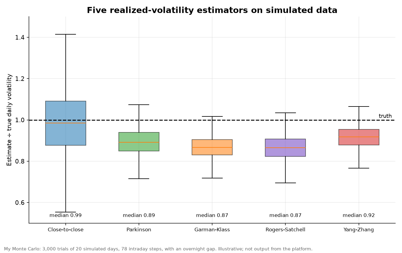
The result is a clean trade-off. The close-to-close estimator was centered on the truth, with a median ratio of 0.99, but it was noisy: the spread of its estimates was about 0.16 of the true value. The range-based estimators were much steadier, with spreads between about 0.055 and 0.065, but they came out low, with medians near 0.87 to 0.89, because they ignore the overnight gap and because a sampled path does not quite touch its true high and low. The Yang-Zhang estimator sat in between, with a median of 0.92 and the smallest spread. This is a simulation under my own assumptions, not output from the platform, and the exact numbers depend on those assumptions. The durable lesson is that “realized volatility” is a choice, and that a platform offering all five lets a researcher see how sensitive a conclusion is to the choice.
The neighboring command computes volatility cones, which show the percentile ranges of rolling realized volatility across several window lengths. A cone is the right answer to the question “is today’s volatility high?” because it compares today’s reading to the history of the same window length.
A note on the technical-versus-quant divide
People often treat technical analysis as one tribe and quantitative analysis as another. This module’s structure suggests a more useful view. A moving average is a linear filter. An oscillator is a normalized difference of filters. A channel is a rolling quantile or a scaled volatility band. Almost everything in the 43 commands is a statistic of a price window, and statistics can be tested. Having the indicators and the testing commands in the same catalog, callable by the same agent in the same pipeline, is what lets a researcher ask the sharper question: not “does this indicator work?” but “does this indicator, on this data, survive a test that accounts for how many indicators I tried?” I will come back to that last clause.
Macro and fixed income: a dashboard you can script
The economy module has 74 commands and the fixed-income module has 34, so about 22 percent of the catalog is about rates, inflation, jobs and the fiscal picture. The reference’s sample captures give a good snapshot of what these commands print, and the data are dated November 17 and 18, 2026.
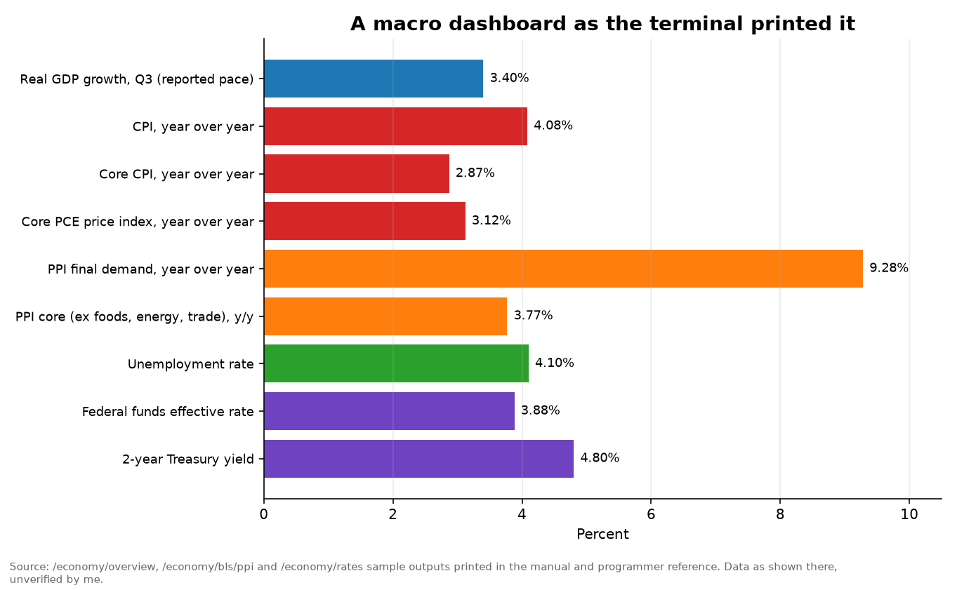
The macro overview returns 16 series. In the portion the documents print, real GDP growth for the third quarter is 3.4 percent, headline consumer prices are up 4.08 percent from a year earlier, core consumer prices are up 2.87 percent, the core personal-consumption price index is up 3.12 percent, the unemployment rate is 4.1 percent, and the effective federal funds rate is 3.88 percent. The producer-price command prints final-demand inflation of 9.28 percent over twelve months and a core measure excluding foods, energy and trade of 3.77 percent, and the rates command shows the two-year Treasury yield at 4.80 percent. These are the values as printed in the PDFs and I have not independently verified them.
A table like this is a good place to practice the discipline of asking whether the numbers hang together. A policy rate of 3.88 percent with a two-year yield of 4.80 percent suggests the market is pricing rate increases, not cuts. A headline CPI of 4.08 percent against a core of 2.87 percent suggests energy and food are doing the heavy lifting. A producer-price headline of 9.28 percent against a core of 3.77 percent suggests the same thing more loudly. None of that is a forecast. It is the kind of cross-reading that a good research agent should do, and the platform makes the inputs easy to fetch in one pipeline.
Fixed-income math you can run offline
The fixed-income module’s offline calculators are my favorite part of the catalog, because they are the pieces a student can verify by hand. Start with the yield curve. The Nelson-Siegel-Svensson model describes the whole curve with six parameters: three for the level, slope and curvature, a fourth for a second hump, and two decay times.
The platform both fits this model to the Treasury curve and evaluates it from parameters you supply. Its sample capture of the fit prints the model name and the first coefficient, and the table has nine rows, but only the first two are printed in the PDF. A bond-pricing command computes a bond’s price from its coupon and yield, along with duration, convexity and DV01, the dollar value of one basis point. Those are defined as follows.
Duration tells you how much the price moves for a small change in yield, and convexity corrects for the curvature. A bond with a modified duration of seven loses roughly seven percent of its price when yields rise by a full percentage point, and a little less than that because of convexity. The DV01 turns the same idea into dollars per basis point, which is how a rates desk sizes a hedge.
The FedWatch commands do something I find elegant. A 30-day federal funds futures contract settles on the average effective rate during its delivery month, and it trades at 100 minus the market-implied average rate. If a month contains a policy meeting, the implied average rate is a day-weighted blend of the rate before the meeting and the rate after it, so the futures price lets you back out the probability of a move.
The reference describes its command as “CME FedWatch meeting probabilities from a 30-Day Fed Funds futures price (offline math),” and a companion command handles a whole strip of contracts across several meetings. I have simplified the equation for exposition: the real calculation weights the days before and after the meeting, and it has to handle meetings that fall at the end of a month. The reference does not print its exact method, so treat my equation as the textbook idea, not as the platform’s code.
The platform also prints inflation breakevens from Treasury inflation-protected securities. The breakeven inflation rate for a maturity is the nominal yield minus the real yield, which is the average inflation rate at which an investor would be indifferent between the two bonds.
The sample capture shows a five-year nominal yield of 4.89 percent and a real yield of 2.66 percent, for a breakeven of 2.23 percent. The seven-year figures are 4.96, 2.76 and 2.20 percent. The two breakevens differ by only three basis points, so the market is not pricing a steep inflation path beyond the five-year point, at least in this capture. Notice the check: 4.89 minus 2.66 is 2.23. The platform’s arithmetic agrees with the definition.
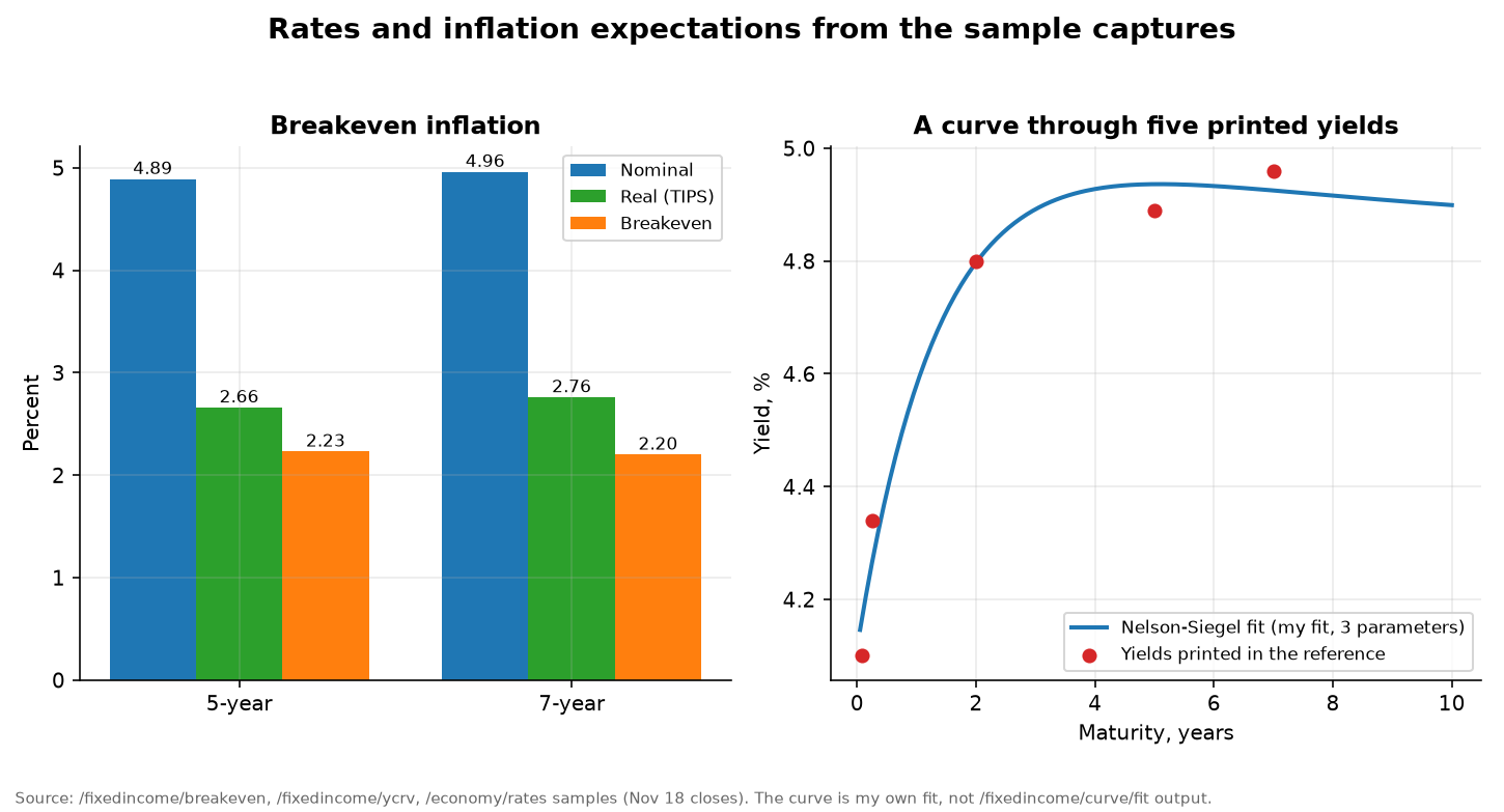
The right panel of the figure takes five printed yields, namely the one-month and three-month Treasury yields from the curve command, the two-year yield from the rates command, and the five-year and seven-year nominal yields from the breakeven command, and passes a three-parameter Nelson-Siegel curve through them. That fit is mine, not the platform’s, and it is there to show what a smooth curve through scattered points looks like. The residuals are all under eight basis points. It is a good reminder that the whole U.S. Treasury curve can be summarized by very few numbers, which is why these models are used for forecasting and for relative-value work.
Other macro, energy, crypto and DeFi captures
The same samples include a few more data points that show the breadth of the catalog. The CBOE term-structure command printed a nine-day volatility index of 23.95 and a one-month index of 24.56 for November 18, down from 26.70 and 25.46 the day before. The put-call ratio on VIX options was 0.88. The Treasury’s debt-to-the-penny command printed total debt of about 40.69 trillion dollars on November 18, split into 32.89 trillion in its public-debt column and 7.80 trillion in its intragovernmental column. The energy commands printed a West Texas Intermediate spot price of 89.53 dollars a barrel and a Brent spot price of 92.94 on November 17, a Henry Hub weekly spot price of 3.03 dollars per million British thermal units, and lower-48 working gas storage of 3,882 billion cubic feet for the week ending November 13.
On the crypto side, the global market command printed Bitcoin dominance of 56.17 percent among 10,956 listed cryptocurrencies. The DeFi commands printed protocol totals and stablecoin supply. I computed one small thing from the stablecoin capture: the largest fiat-backed stablecoin shows 175.07 billion dollars in circulation against 182.72 billion a month earlier, which is a drop of about 4.2 percent, and the second largest shows 68.80 billion against 72.25 billion, a drop of about 4.8 percent. Whether that is a trend or noise is not something I can tell from two rows, and the reference does not claim to tell you. The point is that the catalog lets a single agent assemble a cross-asset morning snapshot, from rates to energy to crypto, in one request.
Futures, FX and options: the derivatives desk in a few dozen commands
The futures and Rithmic modules together hold 37 commands, and the forex module holds 10 more. They split into contract plumbing, which includes contract specifications, the front-month resolver, margin estimates and tick-to-dollar conversion; curve analytics, which includes term structure, calendar spreads, roll yield, carry and basis; options analytics, which includes Black-76 pricing and Greeks, an implied-volatility solver, put-call parity, multi-leg spreads and payoff diagrams; and hedging.
Currency forwards
Covered interest parity ties a currency forward to the spot rate and the two interest rates. The forex module has a command that builds forward rates from money-market rates in this way.
Pricing a futures option
Options on futures are priced with the Black-76 model, which is the Black-Scholes model rewritten so that the underlying is a futures price and carries no cost of carry of its own. The call value and delta are below, with d₁ and d₂ defined inside the equation.
The reference lists a command that prices the option from explicit inputs fully offline, another that returns the Greeks, and another that solves for the implied volatility from a market price using the Newton-Raphson method. Its usage lines list defaults of 20 percent volatility and a 5 percent rate, which I used for the illustration below. The inputs are mine, and no platform output is shown in this figure.
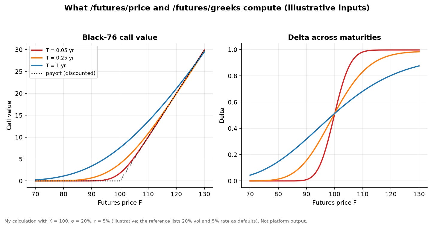
The left panel shows how a call’s value approaches its discounted intrinsic value as expiry nears. The right panel shows the delta, the hedge ratio, steepening into a step function as time runs out. The practical meaning of the right panel is the one every options trader learns the hard way: near expiry and at the strike, delta swings from near zero to near one over a tiny price range, so hedges must be adjusted constantly or accepted as risky. A platform with a Greeks command and a spread-payoff command in the same catalog lets an agent show that to a student in seconds.
Carry, contango and backwardation
The cost-of-carry model says that a futures price should equal the spot price grown at the financing rate and reduced by any yield the holder receives for owning the physical asset, which for commodities is called the convenience yield.
When financing dominates, the curve slopes upward, which traders call contango. When the convenience yield exceeds the financing rate, it slopes downward, which is backwardation. The platform’s carry command compares a deferred contract with this fair value and flags it as rich or cheap, and its curve-signal command classifies the regime and emits a roll bias note.
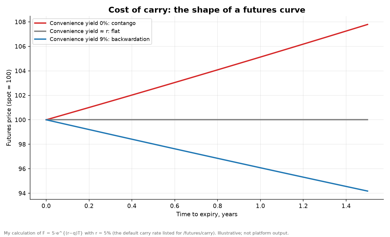
The roll yield is what an investor earns or loses from holding a futures position as it converges to spot, annualized from two points on the curve.
A holder of a long position in contango pays the roll yield, and a holder in backwardation collects it, which is why long-only commodity funds often disappoint relative to spot in contango markets. The platform’s roll command returns the annualized roll yield and the calendar spread, and its term command shows the whole term structure with roll percentages versus the front month.
Hedging with futures
The last equation of this section is the beta-weighted hedge, which tells you how many contracts to short to neutralize an exposure. It scales the portfolio value by its beta and divides by the dollar value of one contract, the futures price times the multiplier.
The platform’s hedge command takes a symbol, a portfolio value and a beta, and returns the contract count. The same module can estimate initial and maintenance margin and convert a move in price points to ticks and dollars per contract. These are the pieces that, strung together in a pipeline, let an agent answer a question like “what would it cost me, in margin and in tick risk, to hedge this exposure?” without a human typing four commands.
The futures data layer
Live futures data come through the Rithmic module, which can connect to a gateway, resolve a root symbol to its front-month contract, list the contract ladder for a root, return contract metadata such as tick size, tick value and multiplier, pull historical candles at daily, weekly or monthly intervals, and collect options chains with Black-76 implied volatilities and Greeks. Several of these work offline, such as the searchable local universe of exchange-listed contracts and the contract-metadata commands. The manual’s own status capture shows the live connection reporting that its configuration is valid but that it is not connected, because the gateway was not running when the manual was generated. That is what an honest status line looks like.
Fundamentals, filings and the equity module
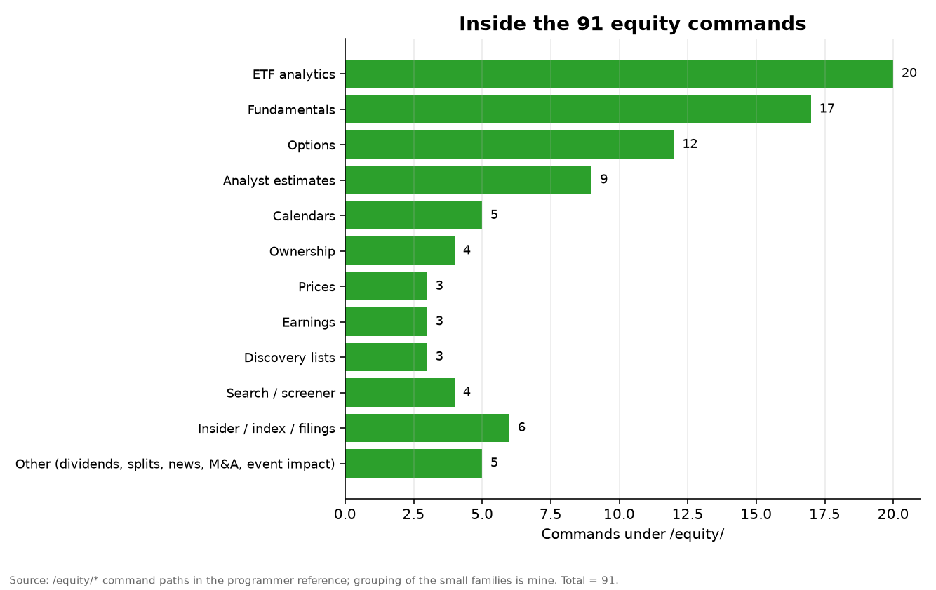
The equity module is the largest, with 91 commands. The biggest block is not stock analysis at all but exchange-traded funds, with 20 commands covering holdings, sector weights, expenses, returns, risk statistics, dividends, regulatory fund portfolios and screeners. Fundamentals follow with 17 commands, options with 12, and analyst estimates with 9.
The options group is worth a short look. It includes a term-structure command that returns, for each expiry, the days to expiry, the at-the-money implied volatility, open interest and volume on calls and puts, and the put-call ratio of open interest. The sample capture prints an at-the-money implied volatility of about 35.8 percent for a contract that expires the same day and about 26.6 percent for one two days out. The difference between those two numbers is not a market view. It is mostly what happens to implied volatility on the final day of an option’s life, when tiny price changes and thin quotes dominate, and it is a nice example of why a term structure is more informative than any one number.
The analyst-estimates commands cover consensus, revisions, trends, rating changes and price targets. The sample capture for one large stock shows a target range starting at 250 dollars with an average of 345.63, and a recommendation breakdown of 6 strong buys, 20 buys, 13 holds, 3 sells and 3 strong sells, for 45 analysts. A research agent can turn that into a one-line summary, but a careful one will also ask how current those ratings are, and the revisions command, which reports estimates now and 7, 30 and 60 days ago, is what answers that question.
From statements to margins
To show what a fundamentals call returns, I used the reference’s own sample for annual revenue and net income for the same large stock, which are printed in the documents as Yahoo-sourced values for fiscal years ending in September.
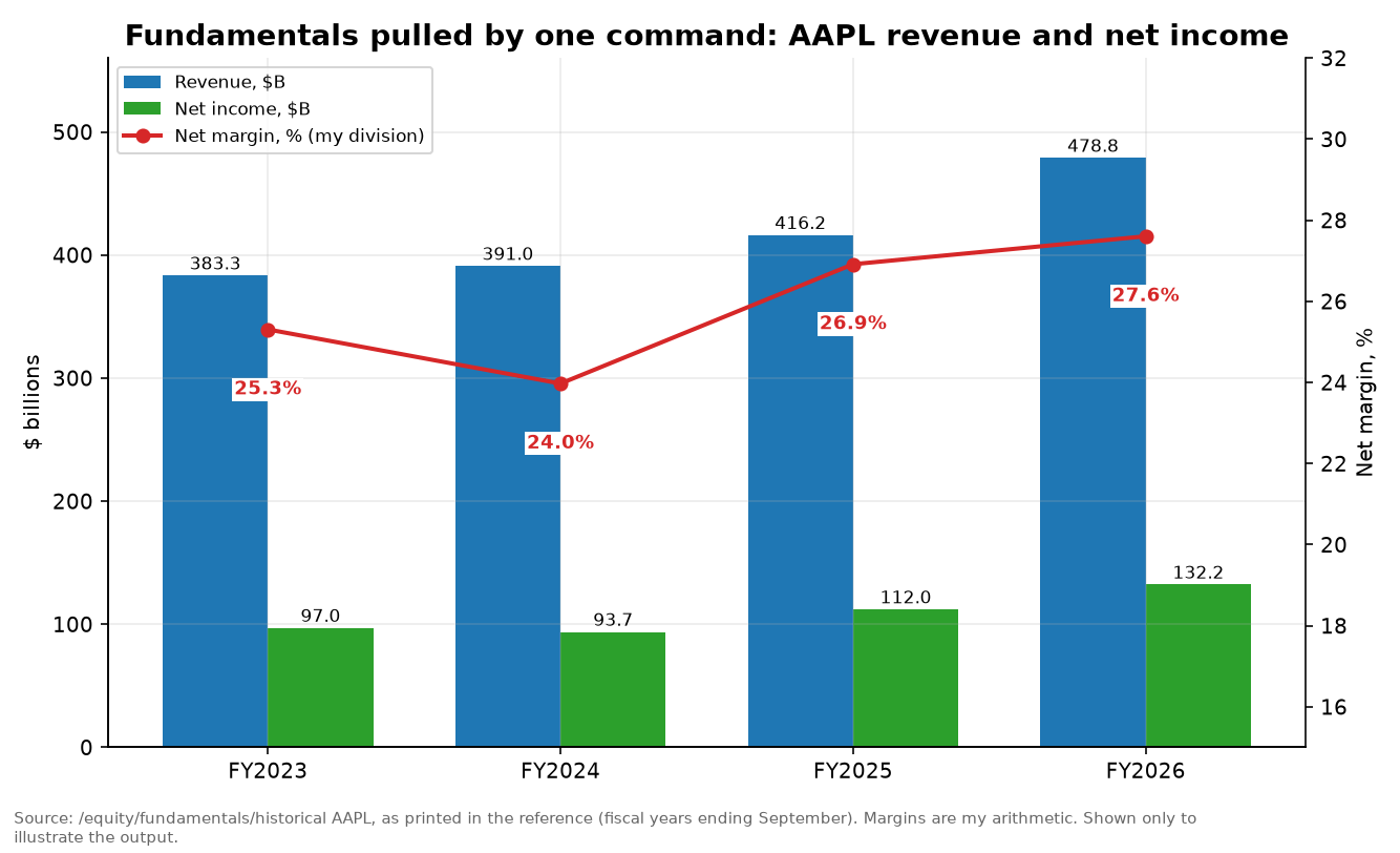
Revenue rises from 383.3 billion dollars in fiscal 2023 to 478.8 billion in fiscal 2026, and net income goes from 97.0 to 132.2 billion. Dividing one by the other gives a net margin of 25.3 percent, 24.0 percent, 26.9 percent and 27.6 percent, which are my arithmetic on the printed values. I am showing this as an example of a command’s output, not as an investment view, and I would not draw a conclusion about a company from two columns of sample data. What the example does show is the shape of the fundamentals toolkit: a statement history from one command, the same history from SEC XBRL filings from another, segment and geographic breakdowns from a third, and growth rates, ratios, shares outstanding and short interest from others, so that an analyst or an agent can cross-check one source against another.
Filings and ownership
The SEC module is a good example of how this platform gives an agent real primary sources. It can search EDGAR’s full text from 2001, list a filing’s exhibits and print one exhibit’s text with the HTML stripped, parse insider transactions from Form 4 filings, show a manager’s 13F history and cover page, pull a mutual fund’s monthly flows and returns from N-PORT filings, and look up an investment adviser or a registered representative in the adviser database. An agent that can read filings itself is much less likely to repeat a rumor than one that can only read headlines, and that is the strongest argument I can make for including these commands in the MCP tool set.
Portfolio construction: where weights come from
The portfolio module has eight commands. They return a full performance and risk scorecard, a rolling market beta, an efficient-frontier sweep with weights at each point, a long-only mean-variance optimization that maximizes the Sharpe ratio or minimizes variance, a performance command that reports Jensen’s alpha, tracking error and the information ratio against a benchmark, and a risk-based allocator with seven methods: equal weight, inverse volatility, equal risk contribution, hierarchical risk parity, its hierarchical equal-risk-contribution variant, maximum decorrelation, and maximum diversification.
The classic problem is to find the weights w that minimize portfolio variance for a given covariance matrix Σ. The risk-parity family changes the question to “what weights make every asset contribute equally to total risk?”
I built a small illustration with four hypothetical assets whose volatilities and correlations I made up, to show how the answers differ. These are not platform outputs, and the inputs have no connection to any real market.
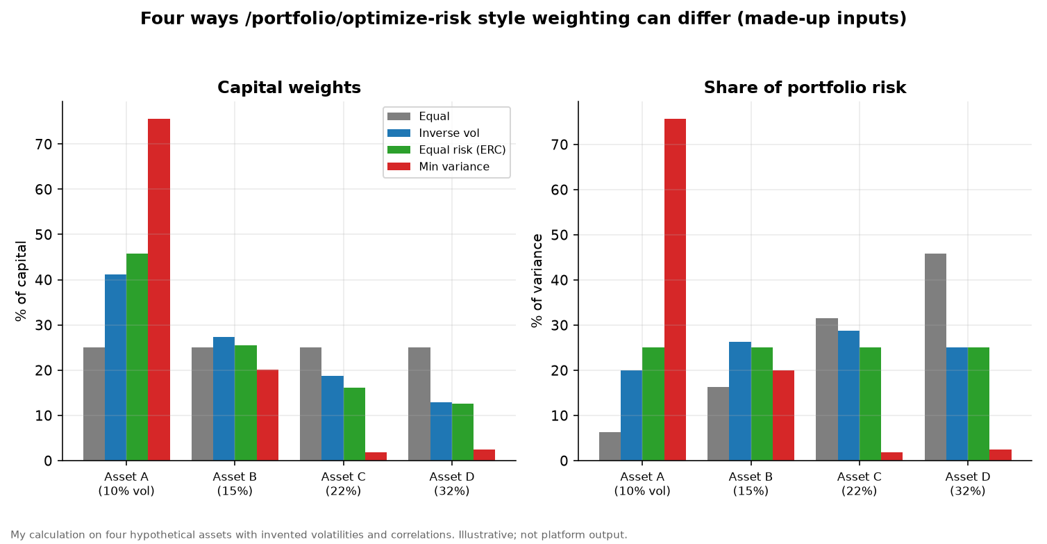
Equal weights give each asset a quarter of the money but give the most volatile one far more than a quarter of the risk. Inverse-volatility weights tilt toward the calm assets. Equal-risk-contribution weights go further and account for correlations, which is why the least volatile asset ends up with about 46 percent of the capital and the most volatile with about 13 percent. The minimum-variance portfolio is the most extreme, putting about three quarters of the capital in the calmest asset and almost nothing in the two riskiest. That concentration is a well-known weakness of minimum-variance optimization, and it is the reason the hierarchical methods exist. A platform that offers all seven methods in one command lets you see how fragile an allocation is to the method you chose.
Backtesting, paper bots and a very short sermon about selection
The backtest module has seven commands: buy and hold, a moving-average crossover test, an SMA-based momentum test, a sector-style rotation test, an RSI test, a trade list, and a what-if comparison of a lump sum against monthly dollar-cost averaging. They take a ticker, some parameters and a transaction-cost input, and print a metrics table.
I want to be precise about my approach to anything involving trading strategies. I am not going to describe the rules, parameters or settings of any strategy, mine or anyone’s, in this article. The documents describe a bot-generation workflow in general terms, and that is all I will discuss here.
What the backtest samples show, and what they should make us do
Here is the part I promised earlier. The reference’s sample captures for the backtest commands, run on the same large stock, print the following total returns: minus 100 percent for buy and hold, minus 100 percent for the moving-average crossover test, minus 100 percent for the momentum test, and plus 210.8 percent for the RSI test. The what-if command prints minus 100 percent for both the lump sum and the monthly purchases. Meanwhile the portfolio-metrics sample for the same stock prints a total return of about plus 118.9 percent.
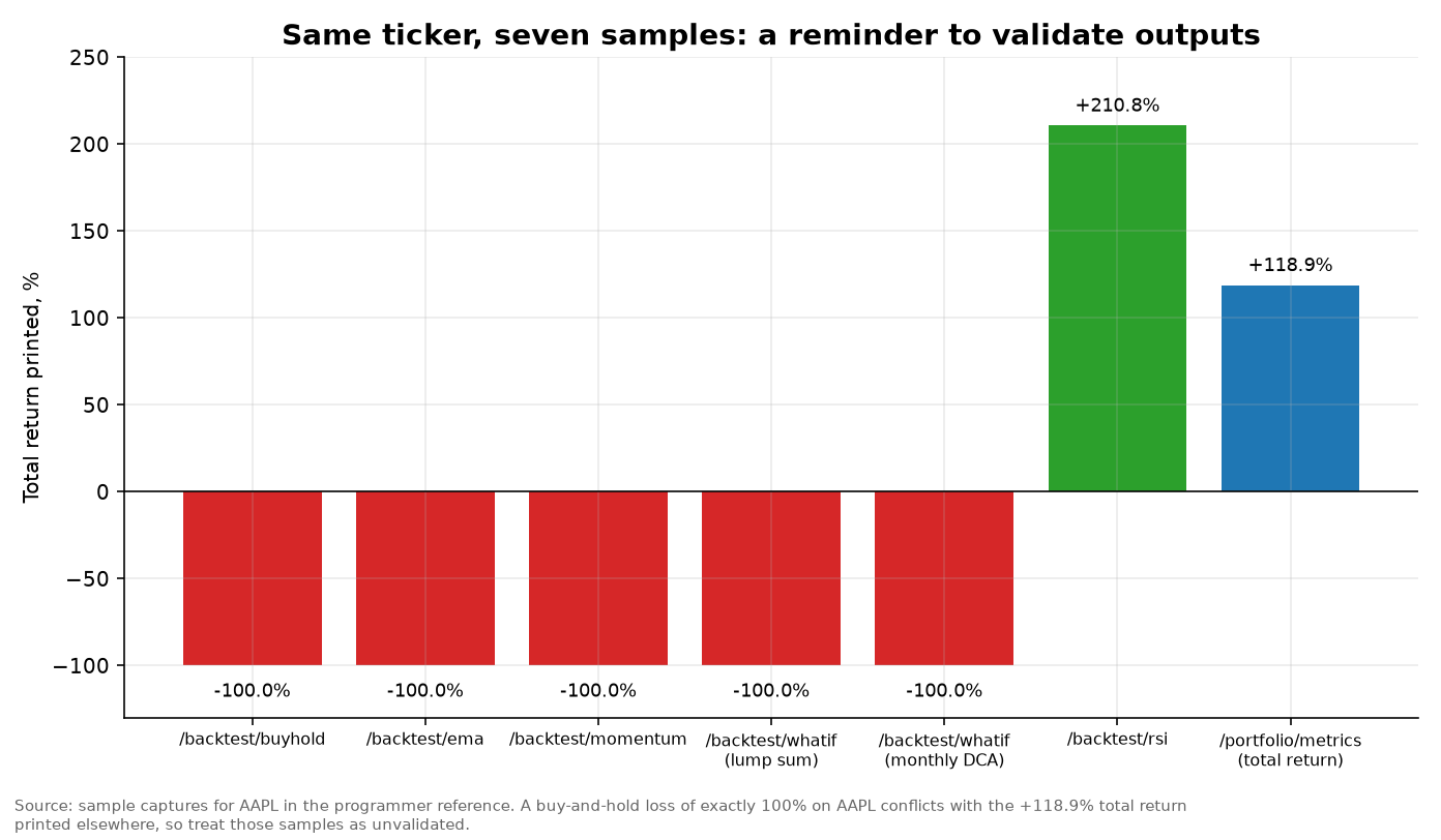
A stock that is down exactly 100 percent has gone to zero. This one printed a 349.21 quote in a capture from the same day. Those two facts cannot both be true, and an agent that read the first sample and wrote “buy and hold lost everything” would be wrong. I cannot tell from the documents why the samples are like this. One of the printed rows is a hint but not proof: the monthly-purchase maximum drawdown prints as minus 40.3157 percent, and the first trade in the trade-list sample entered at a price of 40.315. The closeness of those two numbers makes me suspect a units slip, but that is a guess, and I would like to hear from the people who run the platform.
I am not raising this to score a point. I am raising it because it is the most useful example in either document of how to build agents on top of a research platform. There is an invariant that any buy-and-hold test must satisfy: the gross return should be the final price divided by the first price, minus one, and the net return should be lower than that by the transaction costs. A research agent can verify an invariant like that in a few lines of reasoning before it writes anything. The same goes for “the best Sharpe in this table is above 12,” for “this forecast is half the current price,” and for “this table’s units are unclear.” In pseudocode, the idea looks like this.
for each result the platform returns:
check the invariants that must hold: signs, units, totals, ranges, ordering
compare it with at least one independent command on the same data
if a check fails: say so plainly, quote the numbers, and do not build on the result
else: use it, and cite which command produced it
Platforms improve when agents report discrepancies like this. The fact that the documents are generated from running the program, with the failures left in, is what makes it possible.
Sharpe ratios and the number of things you tried
The second lesson is about selection. A backtest result tells you how an idea did in the past. It does not tell you how many ideas were tried before this one was reported. The Sharpe ratio estimated from n independent trades has a standard error that shrinks only with the square root of n, so the t-statistic is the sample Sharpe ratio times that square root.
Now suppose K strategies with no true edge are each tested, and you report the best. For a Sharpe estimated from n observations, the expected best value of K independent noise strategies grows roughly with the square root of two times the natural log of K.
The platform’s two bot libraries are described in the reference’s samples as 259 bots in the simulation library and 55 entries in the alphamint library, and a ranking command sorts backtested bots by a metric such as Sharpe and returns the top 20 with columns for grade, Sharpe, Sortino, total profit, annualized return and win rate. In the sample ranking I read, one top row shows a Sharpe above 12 with a win rate of 62.5 percent. That percentage equals five wins out of eight, so I would infer that the entry rests on a handful of trades, though the trade count is not printed. A statistic like that is exactly what the next figure is about.
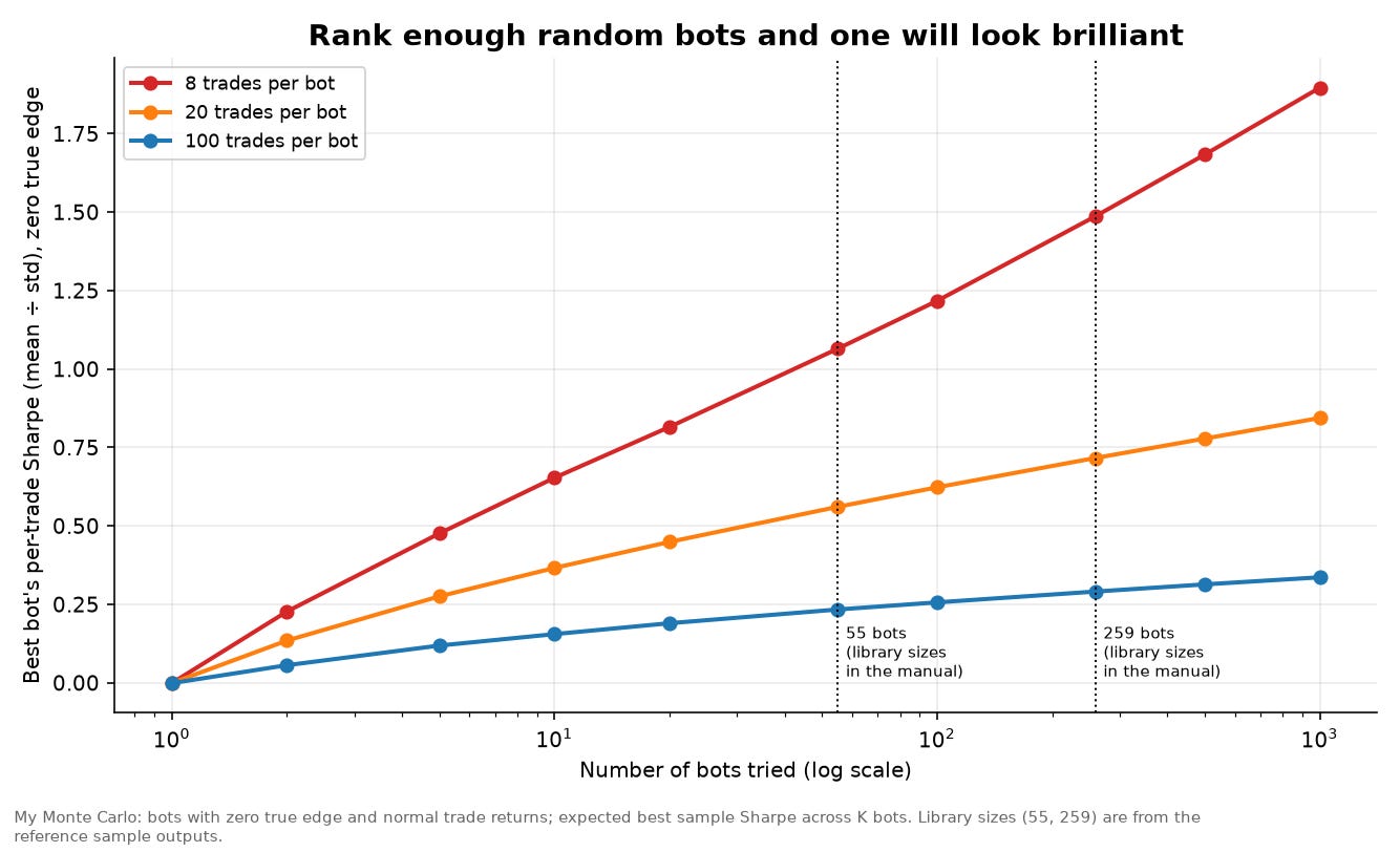
I simulated bots whose true edge is zero, with normally distributed trade results, and recorded the expected best per-trade Sharpe ratio when you pick the best of K. With only 8 trades per bot, the best of 259 zero-edge bots shows a per-trade Sharpe of about 1.5, and the best of 55 shows about 1.1. With 20 trades per bot the figures fall to about 0.72 and 0.56, and with 100 trades to about 0.29 and 0.23. The square-root approximation in the equation slightly understates the small-sample figures, because estimated Sharpe ratios from few observations are fatter-tailed than a normal curve. These are per-trade numbers that cannot be compared directly with an annualized Sharpe in a ranking table, so I am not claiming that any particular ranking row is luck. I am saying that the more bots a library holds and the fewer trades each one has, the more the top of any ranked list is shaped by selection, and that a platform with 259 bots in a library should help its users ask for out-of-sample tests, shorter lists, and adjustments for the number of trials.
The bot workflow, conceptually
The documents describe the Bot pane and a group of 12 bot commands that form a research-to-paper pipeline. At a high level, the platform can take a research report, as a PDF with its source files or as a downloadable archive, and turn it into a set of auditable, paper-only C++ bots plus an article. It can split a Python or text source into separate strategy ideas with one bot each, transpile a Python bot or a folder of bots into a self-contained C++ executable, emit a bot skeleton from a few parameters, and build the generated projects locally. The interface text says the generated projects have no live orders and need no Redis and no broker, and that the report importer does not execute the source files it is given.
The simulation sub-project adds a library of imported paper-trading bots, a ranking command, an offline validator that checks a bot against a set of rules about timeframes, bid and ask handling and mid-price use, and a backtest pipeline that runs in phases and needs the futures gateway session for its data steps. The sample capture of the gateway check prints that it was offline when the reference was generated, which, again, is an honest line. The manual adds that files containing secrets were not copied into the simulation library when it was imported, and that some imported bots contain syntax errors from their source and are listed in a readme, unchanged.
I will say it one more time because it matters: I am deliberately not discussing any individual bot, rule or setting. If you are interested in how a research-to-paper-bot workflow could fit your own process, tell me, and we can talk about it in general terms.
Where this could go: ideas, not promises
I want to be clear about the status of this section. Everything here is my brainstorming, grounded in capabilities the two documents describe. None of it is an announced product, a roadmap, or a promise. I am sharing it because the most useful thing I can do with a platform like this is test ideas against the people who might use it.
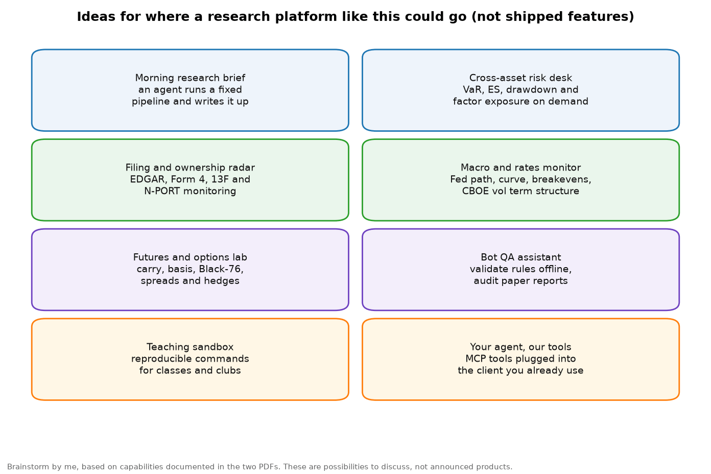
A morning research brief. The agent runs a fixed pipeline each morning: the macro overview, the rates and breakevens, the volatility term structure, energy spot prices, the economic calendar and a few company news searches. It then writes a short summary with every number tied to the command that produced it. The platform already has the commands and the agent loop. What it needs is a standing template and the discipline of the invariant checks I described above.
A cross-asset risk desk. Ask the agent for the value at risk, expected shortfall, drawdown and beta of a list of tickers, along with a risk-parity weighting, and have it explain where the portfolio’s risk comes from. The quant and portfolio commands exist, and the stateless design means each question is a clean, reproducible pipeline.
A filing and ownership radar. Use the SEC commands to watch a list of companies for new insider transactions, institutional holdings changes and filing exhibits, and ask the agent to summarize what changed since last week.
A macro and rates monitor. The FedWatch arithmetic, curve fits, breakevens, term premia and volatility term structure are all offline or keyless. An agent could track how the market-implied policy path and the curve shape move together.
A futures and options lab. Carry, basis, Black-76, spread payoffs and hedge sizing are the building blocks of a desk’s pre-trade analysis, and they work from explicit inputs.
A bot-quality assistant. An agent that runs the offline validator on a bot, compares its paper report with an independent backtest, and checks that the report satisfies basic invariants, without ever being near an order path.
A teaching sandbox. Because every command is reproducible and most are offline, a class or a club could share a set of pipelines and compare results.
Your agent, our tools. Because the MCP server speaks a standard protocol, a user could plug the tools into whichever AI client they already use, rather than switching to a new one.
Questions I would like answered by the people who read this
Which of these appeals to you, and which do you think is a bad idea? What command is missing from the 482? Would you want the agent to explain, to check, or to monitor? Would you rather run it locally, as the documents currently describe, or hosted? And what would make you trust an agent enough to let it work unattended on a research task?
What the documents do not tell me
For completeness, here is what I could not learn from the two PDFs, so that nothing in this article is mistaken for a claim about it. The documents do not state any price, plan, license or terms of service. They do not say how the platform is distributed or whether a hosted version exists. They do not give latency, throughput or capacity figures. They do not describe support, a roadmap or a release schedule. They do not say how third-party data-provider terms apply to your use of those sources, and you should read each provider’s terms yourself. And, as the manual itself says, they did not verify the hosted model service, the broker and futures-gateway connections, the running bots, one MCP transport, the VS Code integration or one C++ example.
If you want to know about any of those things, the right move is to ask rather than assume, and you can ask me directly.
Your turn: what would you like to do with this platform?
Let me end where I started. A research terminal with one catalog of 482 commands, five ways in, an MCP server and a bounded agent loop is an unusual design, and its strongest features are not the flashy ones. It is the single catalog, the stateless processes that make pipelines the unit of analysis, the layered order gates that make unattended agents conceivable, and documentation that prints its own failures.
I would like to hear from you.
Do you want the PDFs? I can email you the 60-page user manual and the 487-page programmer API reference as soon as I can. Send me a direct message on Substack or email me, say that you would like the PDFs, and I will send them.
Do you want to learn more about what is offered? Message me or email me and tell me what you are trying to do. I will tell you what the documents say about it, and I will tell you plainly when they do not say.
And where do you think this goes? Where do you see a platform like this being most useful in the next year, and what would you like to do with it? Leave a comment below, send me a direct message on Substack, or email me. If you are reading this in the Substack app, the message button on my profile is the quickest way. The best answers will shape the next article in this series.
This article is for education and information only. It is not investment advice or a recommendation to buy, sell or hold any security, future, option or digital asset, and it makes no promise of any result. All descriptions of the AlphaMind Terminal platform are drawn from its user manual and programmer API reference as generated on November 19, 2026; I have not independently verified the printed sample outputs, and I describe them as printed. Simulations and illustrations marked as mine use invented or illustrative inputs and are not outputs of the platform. No trading-bot rules, parameters or settings are disclosed here. Futures and options trading involves substantial risk of loss, including losses greater than your initial investment.
Most quantitative research stacks fail because they treat an AI agent as an analyst rather than an unconstrained stochastic proposer 📊.
Handing a language model a toolbox of 480 market endpoints sounds like absolute leverage. In practice, it's an entropy trap. When an agent hops across unbuffered REST calls, it drifts. It drops units. It confuses price differences with percentage returns. It looks at a backtest showing a minus 100% return on a blue-chip equity trading at 350 dollars and writes a fluent three-paragraph explanation for why the business went bankrupt. The prose sounds immaculate. The underlying math is completely detached from reality.
Generative models don't know what an invariant is. They output plausible text. If you want genuine autonomous market research, you must enforce a strict propose-and-commit split ⚖️.
The fix isn't to prompt the model to be more careful. That never works. The real solution is architectural: make every analytical operation completely stateless, and chain executions inside an explicit, deterministic pipeline DAG. The model proposes the recipe: load the asset, compute log returns r_t = ln(P_t / P_{t-1}), calculate 95% Expected Shortfall, and evaluate maximum drawdown. A compiled native process executes the sequence. If a single step violates an algebraic identity, the pipeline terminates immediately with an explicit error. No side effects. No memory pollution. Zero hallucinatory repair.
This structural divide becomes life-or-death the second execution enters the frame 🛑. If you allow an agent anywhere near an order desk, safety cannot depend on model disposition. You need independent, non-bypassable gates across every physical layer. The command flag defaults to dry-run. The configuration rejects live accounts. The network daemon enforces loopback isolation. The tool protocol excludes write permissions by default. When the probability of failure across independent layers is p_i, your joint risk collapses multiplicatively as ∏ p_i. When an operator flips all switches simultaneously, that mathematical shield dissolves into a single point of human failure.
We also need to talk about selection bias in algorithmic strategy generation. When an agent searches through a library of 260 candidate bots and proudly presents an annualized Sharpe ratio of 12, it hasn't discovered an infinite money glitch. It discovered sampling noise. For K independent zero-edge strategies evaluated over n trades, the expected maximum Sharpe ratio naturally scales as E[max_{k ≤ K} SR_k] ≈ √(2 ln K / n) 📈. With eight trades per strategy, pure random variance will hand you a Sharpe above 1.5 every single time.
Here is the core hypothesis we must build our infrastructure around: When analytical workflows exceed 100 tools, autonomous reliability does not scale with parameter size; it scales inversely with state persistence. If an agent operates with zero memory between discrete executions and every proposal is verified by an out-of-band invariant kernel before state mutation, the probability of catastrophic decision drift collapses to zero regardless of model size.
Stop optimizing for conversational sycophancy in financial agents. Build verifiable, hardware-isolated execution boundaries instead 🛡️.
(╯°□°)╯︵ ⋈