


The supplied listing for the 10-Year Treasury Curve Steepener Bot presents an appealing collection of numbers: an estimated 1.71% annualized return, a 1.329 Sharpe ratio, a 2.45 profit factor, and a maximum drawdown of 0.76%.
But the most important sentence appears beneath those figures:
“This specific configuration was not individually backtested.”
That disclosure changes how we should read everything else.
This article examines the supplied Python file, bot_zn_steepener (2)_portable.py, alongside its accompanying product listing. It is a static code review—not a claim that I executed the program, reproduced its results, or verified its trading performance.
The objective is to understand what the strategy actually does, how its components interact, and what would need to change before its results could be evaluated credibly.
There is useful educational material here. There are also missing dependencies, execution assumptions, and several significant bugs.
Studying both is more valuable than repeating a performance headline.
1. Reading the Performance Table Correctly
The listing reports the following figures:
Metric Reported estimate Annualized return 1.71% Sharpe ratio 1.329 Sortino ratio 6.602 Win rate 50.0% Profit factor 2.45 Maximum drawdown 0.76% Grade A
According to the supplied document, these estimates are medians from 12 backtested ZN strategies. They are not measurements from a dedicated backtest of this exact implementation.
The distinction is fundamental.
We cannot say this bot “achieved” a 2.45 profit factor. We can say its listing assigns it a peer-derived estimate of 2.45.
Nor should we treat the metrics as one internally consistent equity curve. A median return, median drawdown, and median Sharpe ratio calculated across several strategies may describe different members of that group.
The source header gives slightly more precision for some values:
# BACKTEST: WinRate=50.0 PF=2.447 AnnRet=1.705%
# (est. from 12 ZN peers)
These comments document an estimate. They do not implement a backtest or establish provenance.
The listing also describes a paper-trading session dated September 25, 2026:
One trade
Zero wins
One loss
Net result: approximately zero dollars
That summary is insufficient to evaluate execution quality or profitability. The apparent mismatch between a losing trade and a displayed zero-dollar result requires the underlying ledger, rounding rules, and trade-classification definitions.
Likewise, the code’s advertised short-term profit potential of $800–$3,200 is not supported by a calculation or strategy-specific result in the supplied materials.
My starting conclusion is therefore narrow:
The performance figures provide context for investigation, not evidence that this exact program has demonstrated an edge.
2. What Does the Strategy Actually Trade?
The configuration is explicit:
BOT_NAME = "10-Year Treasury Curve Steepener Bot"
SYMBOL = "ZNU6"
EXCHANGE = "CBOT"
The constructor specifies:
direction="LONG/SHORT",
num_contracts=5,
signal_timeframe="60m",
execution_timeframe="5m",
The intended structure is a single-instrument, long/short system with hourly signals, five-minute trade management, and a maximum position of five contracts.
However, the strategy’s name is more ambitious than its implementation.
The supplied code does not ingest a two-year yield series, calculate a two-year versus ten-year yield spread, or manage a second trading leg. It also does not identify institutional transactions or measure order flow directly.
Instead, it evaluates one instrument using:
Moving averages
RSI
MACD
Recent trading ranges
Volume
Volatility estimates
Spread and momentum filters
Based on those observable inputs, I would describe it as a single-instrument Treasury futures trend-and-momentum strategy, rather than a demonstrated implementation of a two-leg curve-steepening trade.
That distinction is not cosmetic. It identifies the hypothesis the code actually tests.
There is also a contract-management issue: ZNU6 is hard-coded. Nothing in the supplied file selects successive contracts or implements a roll policy. The listing’s “front-month” label should therefore not be interpreted as an automated contract-selection feature.
3. The Architecture: A Strategy Built Around Missing Infrastructure
The program organizes its work around three major callbacks:
async def on_bar_closed(self, tf_key, bar):
    ...

async def on_market_data(self, data):
    ...

async def on_fill(self, data):
    ...
Their intended responsibilities are reasonably clear.
Hourly bar closes evaluate potential entries. Five-minute bar closes manage existing positions. Market-data updates check stops and produce diagnostics. Fill events are logged.
The problem is that these callbacks belong to a class whose parent is unavailable:
class ZNSteepenerBot(RedisEventDrivenTradingBot):
The import defining RedisEventDrivenTradingBot has been commented out. Consequently, assuming earlier imports succeed, the standalone file fails when Python reaches this class definition.
The missing parent also appears responsible for important functionality:
self.closed_signal_bars
self.closed_execution_bars
self.warmup_gate_ok(...)
self.atr_with_fallback(...)
self.momentum_state()
self.spread_gate(...)
self.start()
self.stop()
These are not merely broker-specific conveniences. Several influence whether a trade occurs and how large it becomes.
The logger factory is missing too. A Redis ping() call remains active, and main() still requires Rithmic credentials.
The listing’s standard-library-only description also conflicts with:
from dotenv import load_dotenv
For publication, I would characterize this package as an incompletely extracted strategy module, not a standalone portable trading application.
A proper repair would replace the missing infrastructure with explicit interfaces for data, execution, clocks, logging, and state management.
4. The Two-Timeframe Design
The code separates entry decisions from position management.
On the signal timeframe, it requires at least 20 closed bars before building a snapshot:
min_bars = 20

warm_ok = self.warmup_gate_ok(
    len(self.closed_signal_bars),
    base_min_bars=min_bars,
    direction="LONG"
)
The execution branch increments a counter and evaluates an open position using shorter-period indicators.
This produces a useful conceptual separation:
The hourly calculation decides whether to enter.
The five-minute calculation decides whether the position remains worth holding.
But the visible handler does not append incoming bars to either history. It assumes another component has already done so.
That creates an integration requirement that should be documented precisely: when on_bar_closed() runs, the corresponding closed-bar collection must already contain the new bar.
Event ordering matters too.
If an hourly bar and a five-minute bar close at the same timestamp, which callback runs first? An hourly signal can use _mid_price(), which prefers the latest execution bar. Different callback ordering could therefore produce different simulated entry prices.
I would make this ordering deterministic and test it explicitly before comparing results between research and paper-trading environments.
5. The Indicator Engine: Understand the Formulas, Not Just the Names
The signal snapshot combines several hand-written indicators:
fast_ma = self._sma(closes, 6)
slow_ma = self._sma(closes, 20)
rsi = self._rsi(closes, 14)
macd_hist = self._macd_hist(closes, 6, 12, 5)
atr_raw = self._atr(bars, 14)
The moving averages are simple arithmetic averages.
Trend direction is defined by their relative positions:
trend_up = fast_ma > slow_ma
trend_down = fast_ma < slow_ma
This is a trend-state condition, not necessarily a fresh crossover. The averages can remain in the same ordering for many bars.
The RSI implementation calculates average gains and losses over the latest 14 changes. It does not recursively smooth those averages.
Its flat-market behavior deserves attention:
if avg_loss <= 0.0:
    return 100.0
A completely unchanged price series has neither gains nor losses, yet this implementation returns 100. That introduces a bullish contribution into the score even though prices have not risen.
The ATR implementation similarly averages recent true ranges directly. Its calculation is transparent, but a replacement library must reproduce that exact convention if the objective is behavioral equivalence.
MACD uses EMA periods of 6 and 12 with a five-period signal line. Each EMA starts from the first available price in the supplied history.
These details are part of the strategy definition. “Uses RSI and MACD” is not enough information to reproduce its signals.
6. Building the Long and Short Scores
The bot converts its indicators into weighted directional scores.
The long score is:
long_score = (
    (20.0 if trend_up else 0.0)
    + 0.30 * rsi_long_score
    + 0.25 * macd_norm
    + 0.15 * breakout_long
    + 0.10 * vol_score
)
The maximum contributions are:
Component Maximum points Trend alignment 20 RSI 30 MACD 25 Range position 15 Volume 10
The short score mirrors the directional components.
This is an interpretable design: a developer can inspect the score and see which inputs contributed to a decision.
But its “breakout” terminology needs qualification.
The channel includes the current bar:
donchian_high = max(highs[-20:])
donchian_low = min(lows[-20:])
For valid OHLC data, the latest close cannot exceed its own high. Since that high is included in the channel, close >= donchian_high generally requires equality at the highest high.
More importantly, an actual breakout is not mandatory. Prices inside the channel still receive positive scores based on their location within the range.
The listing therefore overstates matters when it describes Donchian breakout as a required entry condition.
If the intended hypothesis were a close above the previous 20 bars’ highs, I would instead calculate the channel from a window excluding the current bar. That would be a strategy change, however—not merely a cosmetic correction.
7. Entry Gates: A Signal Is Only the Beginning
Before entering, the bot checks more than its directional score.
The visible sequence includes:
Warmup completion
Market-data freshness
Bid/ask spread acceptability
Session restrictions
Trading-enabled configuration
Circuit-breaker status
Directional and momentum conditions
Position-size eligibility
A trade-risk ceiling
A cumulative-profit threshold
This layered structure makes the decision process easier to diagnose.
For example, freshness starts with:
stale_age = (
    now - self.last_market_data_ts
).total_seconds()
But last_market_data_ts is set using local receipt time, not a timestamp supplied by the market-data event.
An old observation delivered now could therefore appear fresh. I would track both exchange-event time and local receipt time.
The long and short conditions also share this requirement:
momentum_score >= 50.0
Whether that makes sense depends on the missing momentum_state() implementation. The score could represent direction-neutral strength—or it could encode bullishness. The visible file does not resolve that ambiguity.
Likewise, the spread threshold incorporates a rolling percentile of observed spreads. That is adaptive, but it can also relax the threshold as observed spreads widen.
My proposed revision would separate an adaptive threshold from an independently configured maximum acceptable spread.
8. ATR Stops and the So-Called VIX Proxy
The initial stop distance is:
stop_distance = max(
    atr * atr_mult,
    self.min_stop_ticks * self.tick_size
)
The default minimum is five ticks.
The file sets the point value to $1,000 and tick size to 0.015625. These correspond to CME’s published outright ten-year Treasury-note futures pricing increments: one sixty-fourth of a point, worth $15.625 per contract. (cmegroup.com)
Using the file’s defaults, a five-tick distance represents:
5 × 0.015625 × $1,000 = $78.125 per contract
That is a price-distance calculation, not a guaranteed maximum realized loss.
The ATR multiplier depends on a variable called vix_proxy:
return max(
    10.0,
    min(60.0, (atr / mid) * 10000.0)
)
No VIX observations enter this calculation. It is a bounded transformation of ATR relative to price.
Its purpose is still understandable: adjust stops and sizing according to the instrument’s recent movement. But I would rename it atr_regime_score to avoid implying that an external volatility index is being measured.
The multipliers are:
Below 15: two times ATR
From 15 through 25: 2.5 times ATR
Above 25: three times ATR
The thresholds create discrete changes. I would test behavior immediately around each boundary, rather than assuming the labels describe meaningful market regimes.
9. Position Sizing—and a Units Mismatch
The initial sizing calculation follows a recognizable structure:
base_contracts = (
    self.account_capital * risk_percent
) / max(
    self.tick_size * self.point_value,
    stop_distance
    * self.contract_multiplier
    * self.point_value
)
In simplified form:
Contracts = Risk budget / Dollar stop distance per contract
The code then applies volatility, regime, and momentum adjustments before truncating to an integer and enforcing the five-contract cap.
The questionable step is the volatility baseline:
baseline_atr = max(
    self.tick_size * self.min_stop_ticks,
    self._sma(list(self.vol_history), 20) or atr
)
vol_history contains standard deviations of percentage returns. ATR is measured in price points.
Those quantities have different units, yet the next calculation divides the baseline by ATR as though they were directly comparable.
That makes the adjustment difficult to interpret.
My preferred repair would be to choose one consistent representation:
Maintain a separate history of ATR values; or
Compare normalized ATR values throughout.
The “portfolio risk” check also deserves a more accurate name. It compares the proposed position’s stop-distance risk with 6% of configured account capital. It does not aggregate other strategies, positions, or correlated exposures.
Finally, account_capital remains a configured number in the visible implementation. It does not automatically rise or fall with simulated equity.
These are assumptions to document before interpreting any sizing-based performance result.
10. Scaling Out at 1R, 2R, and 3R
The strategy defines one R as its initial stop distance.
For a long position:
move = mid - self.sim_entry_price
The execution handler then considers partial exits at one, two, and three times that distance.
For five contracts, _build_scale_out_plan() produces:
[2, 1, 2]
That means:
Two contracts allocated to 1R
One allocated to 2R
Two allocated to 3R
Assuming exact fills at those levels, the weighted result would be:
(2 × 1R + 1 × 2R + 2 × 3R) / 5 = 2R
This is illustrative arithmetic, not an observed outcome.
There is also a mismatch between the displayed target and the exit mechanism.
At entry, the bot calculates:
self.current_target_price = (
    entry_price + stop_distance * rr_ratio
)
But the visible exit logic does not check that target price. It uses fixed R-multiple scale-outs, stops, invalidation, and time exits.
Consequently, changing the dynamic rr_ratio does not directly move the actual scale-out thresholds.
The strategy’s advertised reward-to-risk validation is therefore weaker than it appears: it validates a calculated target that is not the operative profit-taking rule.
11. A Critical Bug: Small Positions Can Freeze the Program
The scale-out allocator assumes all three exit stages must receive at least one contract.
That is impossible when the position contains only one or two contracts.
The function eventually reaches:
while half + quarter + rem > qty:
    if half > 1:
        half -= 1
    elif quarter > 1:
        quarter -= 1
    else:
        rem = max(1, rem - 1)
For qty=1 or qty=2, all three buckets can become one. Their sum remains three, but none can fall below one.
The loop never terminates.
This is especially significant because the sizing logic explicitly allows one- and two-contract entries.
The allocator runs synchronously inside an asynchronous entry method. Python’s documentation explains that blocking computation in an event-loop thread delays the other tasks and I/O using that thread. Here, a nonterminating loop could prevent subsequent stop checks and telemetry from running. (docs.python.org)
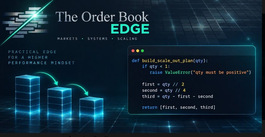
One illustrative repair is to allow empty stages:
def build_scale_out_plan(qty):
    if qty < 1:
        raise ValueError("qty must be positive")

    first = qty // 2
    second = qty // 4
    third = qty - first - second

    return [first, second, third]
However, the caller must also skip zero-sized stages. The existing _simulate_exit() forces requested quantities to at least one, so replacing only the allocator would introduce unintended exits.
This is a useful example of why a local fix needs integration tests.
12. The Fill Model Is the Largest Research Concern
The function named _mid_price() usually returns:
(high + low) / 2.0
from the most recent closed execution bar.
It does not normally return the current bid/ask midpoint.
That price becomes the basis for simulated entries, exits, unrealized profit, and some management decisions.
Consider an illustrative sequence:
The latest closed bar has a high of 112.00 and low of 111.50.
_mid_price()therefore returns 111.75.A subsequent market update arrives at 111.25.
That update triggers a long-position stop.
_simulate_exit()still obtains its price from_mid_price().
The simulated exit can therefore be recorded at 111.75 rather than near the triggering observation.
The problem is not that this always improves results. The problem is that the recorded fill is disconnected from the event that caused the exit.
Entry pricing has a related weakness. A signal decided after a bar closes cannot simply assume execution at that completed bar’s range midpoint.
I would separate four concepts:
Indicator reference price
Position-marking price
Order trigger price
Executed fill price
For a revised simulator, I would define fills using subsequent executable observations, explicit side-dependent pricing, and disclosed costs.
The supplied code does not currently make those distinctions.
13. Stops, Trailing Logic, and Holding Periods
The initial stop remains fixed after entry. A separate trailing stop tightens as the position moves favorably.
For a long:
proposed = mid - trail_distance

self.current_trailing_stop = max(
    self.current_trailing_stop,
    proposed
)
For a short, the corresponding calculation uses min().
That preserves a useful invariant: the trailing stop does not move away from the position in this update logic.
However, the proposed level is based on the closed-bar range midpoint, not a favorable intrabar extreme.
Stop triggering occurs in on_market_data(), while trailing updates occur in the execution-bar handler. A bars-only integration would therefore omit the current stop-triggering mechanism unless it explicitly recreated it.
The code also exits when short-term indicators invalidate the position:
fast = self._sma(closes, 3)
slow = self._sma(closes, 6)
macd_h = self._macd_hist(closes, 3, 6, 3)
A long can be closed when the fast average falls below the slow average or the MACD histogram turns negative.
Finally, the holding threshold ranges from five to 20 execution bars. With the configured five-minute timeframe and uninterrupted bars, that corresponds to approximately 25–100 minutes.
The threshold is recalculated during management rather than fixed at entry, so the effective deadline can change with volatility.
14. Circuit Breakers That Do Not Reset
The bot tracks realized profit by day and week, alongside consecutive losing exit records.
It activates a breaker when:
Daily realized P&L breaches its limit
Weekly realized P&L breaches its limit
Consecutive losses reach five
The major defect is the lifecycle of:
self.circuit_breaker_active
The visible code sets it to True, but never resets it to False.
Moreover, when the breaker is active, _check_circuit_breakers() assigns a cooldown ending at the next calculated midnight. Repeated checks can continue moving that deadline forward.
This is not a complete “pause until tomorrow” mechanism.
I would model breaker reasons separately. A daily-loss halt, weekly-loss halt, and operational failure do not necessarily deserve the same reset policy.
Timekeeping also needs revision. The code approximates Eastern time by subtracting four hours from UTC. Python’s zoneinfo supports named IANA time zones and daylight-saving transitions, making an explicit conversion a better foundation:
from zoneinfo import ZoneInfo

et_now = ts_utc.astimezone(
    ZoneInfo("America/New_York")
)
Timezone data must be available on the deployment system; cross-platform deployments may need the tzdata package. (docs.python.org)
Even that does not define the trading session. I would separately specify session boundaries, holiday handling, and which session owns overnight P&L.
The current daily and weekly limits also monitor realized results, not a complete marked-to-market loss measure.
15. Trade Statistics Need Clear Accounting Definitions
Every partial exit appends a record to sim_trades.
The rolling statistics then treat those records as trades:
wins = [
    t for t in self.sim_trades[-50:]
    if t.get("pnl", 0.0) > 0.0
]
A single entry closed in three portions can therefore contribute three observations.
This affects:
Win rate
Consecutive-loss counting
Profit factor
Dynamic reward-to-risk settings
The dynamic cumulative-profit threshold
The internal variable called sharpe is:
sharpe = mean / std
Here, mean and std come from dollar P&L on recent exit records. The calculation has no return normalization, elapsed-time treatment, or annualization.
It should not be equated with the listing’s reported Sharpe ratio.
There is another edge case: when gross losses are zero, the code returns gross profit as its “profit factor.” That substitutes a dollar amount for a ratio.
I would keep separate datasets for fills, partial exits, completed positions, and portfolio returns. Each answers a different question.
The “session target” also uses lifetime sim_cumulative_pnl, with no visible daily reset. Once reached, it can block future entries across sessions while that state persists.
Names should describe actual accounting behavior, not intended behavior.
16. What a Credible Backtest Would Require
Before optimizing indicator periods, I would establish a reproducible research environment.
Make the strategy executable
Replace the missing parent class, logger, bar storage, and helper methods with explicit implementations. Remove obsolete credential checks and Redis calls.
Introduce an injectable clock
The program repeatedly calls:
datetime.now(timezone.utc)
A historical replay needs strategy decisions to use replay time, not the computer’s present wall clock.
Otherwise, session keys, holding timestamps, cooldowns, and freshness checks can describe the wrong period.
Specify the market-data contract
Document timestamp conventions, bar-close ordering, missing-data handling, quote fields, contract selection, and roll treatment.
Define fills and costs
State exactly when an order becomes eligible to fill, which observation supplies its price, and how commissions, spread, and slippage are represented.
Test invariants
My initial test list would include:
Scale-out quantities sum to the original position.
Zero-sized stages never create an exit.
One- and two-contract positions never hang.
Stops use the intended trigger and fill observations.
Breakers reset only under their defined conditions.
Partial exits cannot reverse a position.
Realized P&L reconciles with the fill ledger.
Replaying identical data produces identical decisions.
Evaluate the exact repaired version
Only then would I calculate strategy-specific returns, drawdowns, win rates, and risk-adjusted statistics.
I would also preserve the source version and configuration behind every run. Fixing the execution model or changing the channel definition creates a materially different experiment.
The result should be a reproducible ledger and equity curve—not simply another performance table.
Conclusion: The Useful Lesson Is in the Implementation
This bot contains several worthwhile design ideas: separate signal and management timeframes, explicit directional scores, volatility-aware sizing, partial profit-taking, tightening trailing stops, and structured diagnostics.
It also illustrates how easily a strategy description can get ahead of the software.
The supplied file is not independently runnable. Its advertised performance is borrowed from peer strategies. Its curve-steepener label is not supported by a visible curve calculation. Its scale-out allocator can hang, its breaker lacks a reset path, and its simulated fills can use stale bar-derived prices.
None of that proves the underlying trading hypothesis is worthless.
It means the hypothesis has not yet been cleanly isolated and tested in the supplied implementation.
For a developer, that is the real opportunity: turn implicit assumptions into explicit rules, repair the state transitions, define execution honestly, and produce results that someone else can reproduce.
A backtest headline invites attention. A reproducible implementation earns confidence.
Educational purposes only. This article analyzes supplied software and reported estimates; it does not establish profitability or recommend trading the strategy with real capital.