


Most quantitative finance resources perpetuate a convenient fiction: financial engineering is treated as an exercise in clean data wrangling, abstract matrix transformations, and frictionless execution. In backtesting notebooks, trades occur on zero-latency continuous midpoints, margin is an afterthought, and the mechanics of the broker interface are abstracted away into hypothetical fill functions.
When deploying automated trading systems into production—especially within regulated futures markets like the Chicago Mercantile Exchange (CME) via the Interactive Brokers (IBKR) Trader Workstation (TWS) API—this academic abstraction collapses:
Exchange Microstructure Constraints: Calculated continuous theoretical prices are rejected by exchange matching engines because they do not conform to discrete minimum tick sizes (e.g., $5.00 index points on CME Micro Bitcoin).
Network Threading & Event Queues: Background network sockets running over TCP will choke if pricing computations block the broker’s incoming message thread.
Ambiguous State Spaces: Dropped packets and socket disconnects (e.g., IBKR error codes
1100,1101,1102) leave order lifecycles stranded in local memory, creating catastrophic directional risk if not reconciled against the broker’s central ledger.Numerical Instabilities in Volatility Solvers: Standard iterative root-finders (such as unbounded Newton-Raphson) diverge into NaN or infinite loops when pricing out-of-the-money options where Vega approaches zero.
To address the gap between derivative modeling and real-world C++ execution, HFTCODE released a detailed 59-page architectural blueprint and reference codebase: Bitcoin Futures, Volatility Analytics & IBKR Integration — C++17 Technical Guide & Code Architecture (PDF). The manual includes complete, zero-dependency C++17 header implementations (CryptoAnalytics.hpp and CryptoSession.hpp), state machine specifications, and pre-trade margin gates.
Below is an end-to-end technical breakdown of the architecture, where every mathematical formula, pricing equation, and execution algorithm is cast into rigorous pseudocode pointing directly to the production implementations documented in the guide.
1. Derivative Economics, Tick Boundaries, and Pre-Trade Risk Gates
Institutional Bitcoin trading on CME diverges significantly from trading spot crypto or retail perpetual swaps (perpsperpsperps). Perpetual swaps rely on continuous funding rates and stablecoin collateral, whereas CME contracts are standardized, cash-settled derivatives expiring against the CME CF Bitcoin Reference Rate (BRR).
Contract Multiplier and Notional Discrepancies
A primary trap for automated systems is failing to distinguish between the standard contract (BTC) and the Micro contract (MBT):
Standard Bitcoin Futures (
BTC): 5.0 Bitcoin multiplier. At $70,000/BTC, one contract controls $350,000 in notional exposure.Micro Bitcoin Futures (
MBT): 0.10 Bitcoin multiplier. At $70,000/BTC, one contract controls $7,000 in notional exposure.
Both trade in minimum fluctuations of 5.00 index points. For MBT, each tick represents:
Tick Value=5.00×0.10=$0.50 USD\text{Tick Value} = 5.00 \times 0.10 = \$0.50 \text{ USD}Tick Value=5.00×0.10=$0.50 USD
Passive Tick-Rounding Engine
Sending raw floating-point prices calculated from theoretical models results in broker rejections. The execution engine must map continuous prices to discrete tick increments while strictly maintaining passive execution intent (avoiding crossing the book unintentionally).
// ============================================================================
// PSEUDOCODE: DISCRETE TICK BOUNDARY SNAPPING
// Reference Implementation: CryptoAnalytics.hpp & CryptoSession.hpp
// Guide: https://hftcode.com/products/bitcoin-futures-volatility-analytics-ibkr-integration-c-17-technical-guide-code-architecture-pdf
// ============================================================================

FUNCTION SnapToValidTick(raw_price, tick_size, order_side)
    INPUT:
        raw_price   : REAL    // Raw model output (e.g., 67423.472)
        tick_size   : REAL    // Minimum tick fluctuation (e.g., 5.00)
        order_side  : ENUM    // BUY_SIDE, SELL_SIDE, or MID_POINT
    OUTPUT:
        valid_price : REAL    // Exchange-compliant discrete price

    IF tick_size <= 0.0 THEN
        TRIGGER_FATAL_ERROR("Invalid tick size specified for contract.")
    END IF

    // Scale raw price by tick increment
    scaled_ticks <- raw_price / tick_size

    MATCH order_side WITH
        CASE BUY_SIDE:
            // Round downward (floor) to prevent accidentally lifting the ask
            discrete_ticks <- INTEGER_FLOOR(scaled_ticks)

        CASE SELL_SIDE:
            // Round upward (ceil) to prevent accidentally hitting the bid
            discrete_ticks <- INTEGER_CEIL(scaled_ticks)

        CASE MID_POINT:
            // Standard nearest-tick rounding for fair-value evaluation
            discrete_ticks <- INTEGER_ROUND_NEAREST(scaled_ticks)
    END MATCH

    valid_price <- discrete_ticks * tick_size
    RETURN valid_price
END FUNCTION
Dynamic Pre-Trade Margin and Notional Safety Gate
Margin requirements on CME futures are non-linear and subject to broker-specific maintenance buffers. Before dispatching any order to the network socket, the state engine must evaluate available liquidity under adverse shock assumptions.
// ============================================================================
// PSEUDOCODE: PRE-TRADE NOTIONAL AND MARGIN GATE
// Reference Implementation: Section 1 & Section 4 Risk Gates
// Guide: https://hftcode.com/products/bitcoin-futures-volatility-analytics-ibkr-integration-c-17-technical-guide-code-architecture-pdf
// ============================================================================

FUNCTION EvaluatePreTradeRisk(account_equity, current_maintenance_margin,
                              target_order, contract_multiplier,
                              initial_margin_rate, max_notional_limit)
    INPUT:
        account_equity             : REAL  // Total net liquidation value
        current_maintenance_margin : REAL  // Currently absorbed margin
        target_order               : STRUCT { quantity: INT, limit_price: REAL }
        contract_multiplier        : REAL  // 0.10 for CME MBT
        initial_margin_rate        : REAL  // e.g., 0.35 for 35% margin requirement
        max_notional_limit         : REAL  // Account ceiling for single-instrument exposure
    OUTPUT:
        risk_passed                : BOOLEAN

    // Calculate incremental notional exposure
    incremental_notional <- target_order.quantity * target_order.limit_price * contract_multiplier

    // Check account-level notional ceiling
    IF incremental_notional > max_notional_limit THEN
        LOG_WARNING("Risk Gate Rejected: Order notional exceeds absolute ceiling.")
        RETURN FALSE
    END IF

    // Compute required capital reserves
    projected_margin_add <- incremental_notional * initial_margin_rate
    projected_total_margin <- current_maintenance_margin + projected_margin_add

    // Enforce an unencumbered cash buffer (e.g., 20% liquid cushion)
    required_cushion <- account_equity * 0.20
    available_liquidity <- account_equity - projected_total_margin

    IF available_liquidity < required_cushion THEN
        LOG_WARNING("Risk Gate Rejected: Available margin buffer falls below safety threshold.")
        RETURN FALSE
    END IF

    RETURN TRUE
END FUNCTION
2. Quantitative Volatility Pipeline and Pricing Engine (CryptoAnalytics.hpp)
The mathematical module in a production execution architecture must run with zero external library bloat, avoiding dynamic heap allocations on the hot execution path. The HFTCODE guide isolates these analytical models within a self-contained C++17 header (CryptoAnalytics.hpp).
+---------------------------------------------------------------------------------+
|                       CRYPTOANALYTICS MATHEMATICAL PIPELINE                     |
+---------------------------------------------------------------------------------+
|                                                                                 |
|  Price Stream (P_t) ---> [ComputeDemeanedRealizedVol] ---> High-Frequency Sigma |
|          |                                                                      |
|          +-------------> [UpdateEWMAVariance]        ---> Hot-Path Dynamic Vol  |
|                                                                                 |
|  Futures Chain (F, K) -> [Black76_OptionPrice]       ---> Fair Theoretical Value|
|          |                                                                      |
|          +-------------> [Black76_AnalyticalGreeks]  ---> Dynamic Risk (Δ, Γ, ν)|
|          |                                                                      |
|          +-------------> [SolveImpliedVolBisection]  ---> Vol Surface / Basis   |
|                                                                                 |
+---------------------------------------------------------------------------------+
Realized Volatility: Demeaned Log Returns
For high-frequency intraday price feeds, calculating a rolling mean introduces unnecessary sampling variance. High-frequency models assume a zero-mean return over short horizons.
// ============================================================================
// PSEUDOCODE: DEMEANED REALIZED VOLATILITY ESTIMATOR
// Reference Implementation: CryptoAnalytics.hpp
// Guide: https://hftcode.com/products/bitcoin-futures-volatility-analytics-ibkr-integration-c-17-technical-guide-code-architecture-pdf
// ============================================================================

FUNCTION ComputeDemeanedRealizedVol(price_series, annualization_scalar)
    INPUT:
        price_series         : ARRAY OF REAL // Sequence of tick/bar prices [P_0, ..., P_N]
        annualization_scalar : REAL          // e.g., 365.0 for 24/7 crypto markets
    OUTPUT:
        annualized_sigma     : REAL

    N <- LENGTH(price_series)
    IF N < 2 THEN
        RETURN 0.0
    END IF

    sum_squared_returns <- 0.0

    FOR i FROM 1 TO (N - 1) DO
        IF price_series[i] <= 0.0 OR price_series[i - 1] <= 0.0 THEN
            TRIGGER_FATAL_ERROR("Non-positive price encountered in return calculation.")
        END IF

        // Compute logarithmic return
        r_i <- LOG_NATURAL(price_series[i] / price_series[i - 1])

        // Accumulate squared returns assuming zero drift
        sum_squared_returns <- sum_squared_returns + (r_i * r_i)
    END FOR

    sample_variance <- sum_squared_returns / (N - 1)
    annualized_sigma <- SQUARE_ROOT(sample_variance * annualization_scalar)

    RETURN annualized_sigma
END FUNCTION
Exponentially Weighted Moving Average (EWMA) Volatility
In tick-by-tick monitoring, rolling window buffers require maintaining dynamic memory. RiskMetrics-style EWMA models update in O(1)O(1)O(1) constant time with minimal state overhead:
// ============================================================================
// PSEUDOCODE: O(1) EWMA VARIANCE TRACKER
// Reference Implementation: CryptoAnalytics.hpp
// Guide: https://hftcode.com/products/bitcoin-futures-volatility-analytics-ibkr-integration-c-17-technical-guide-code-architecture-pdf
// ============================================================================

FUNCTION UpdateEWMAVariance(previous_variance, current_price, previous_price, decay_lambda)
    INPUT:
        previous_variance : REAL // Last computed variance (sigma_{t-1}^2)
        current_price     : REAL // Latest futures price (P_t)
        previous_price    : REAL // Prior tick price (P_{t-1})
        decay_lambda      : REAL // Smoothing parameter (e.g., 0.94)
    OUTPUT:
        new_variance      : REAL // Updated variance (sigma_t^2)

    IF current_price <= 0.0 OR previous_price <= 0.0 THEN
        RETURN previous_variance
    END IF

    log_return <- LOG_NATURAL(current_price / previous_price)
    squared_shock <- log_return * log_return

    // Recurrence relation: sigma_t^2 = lambda * sigma_{t-1}^2 + (1 - lambda) * r_t^2
    new_variance <- (decay_lambda * previous_variance) + ((1.0 - decay_lambda) * squared_shock)

    RETURN new_variance
END FUNCTION
Black-76 Valuation for Futures Options
Equity option equations assume funding costs on cash spot assets. In futures markets, capital is not deployed upfront to purchase the underlying asset (margin deposits earn interest or are backed by Treasuries). We therefore use Fischer Black’s 1976 model (Black-76).
// ============================================================================
// PSEUDOCODE: BLACK-76 CLOSED-FORM VALUATION
// Reference Implementation: CryptoAnalytics.hpp
// Guide: https://hftcode.com/products/bitcoin-futures-volatility-analytics-ibkr-integration-c-17-technical-guide-code-architecture-pdf
// ============================================================================

FUNCTION Black76_OptionPrice(call_or_put, futures_price, strike_price,
                             time_to_expiry, risk_free_rate, volatility)
    INPUT:
        call_or_put    : ENUM    // OPTION_CALL or OPTION_PUT
        futures_price  : REAL    // Underlying forward/futures price (F)
        strike_price   : REAL    // Strike price (K)
        time_to_expiry : REAL    // Annualized time fraction (T)
        risk_free_rate : REAL    // Constant risk-free rate (r)
        volatility     : REAL    // Annualized volatility (sigma)
    OUTPUT:
        option_value   : REAL

    // Guard against non-economic parameters
    IF futures_price <= 0.0 OR strike_price <= 0.0 OR time_to_expiry <= 0.0 OR volatility <= 0.0 THEN
        RETURN 0.0
    END IF

    vol_sqrt_t <- volatility * SQUARE_ROOT(time_to_expiry)

    // Evaluate normalized distribution parameters d1 and d2
    d1 <- (LOG_NATURAL(futures_price / strike_price) + (0.5 * volatility * volatility * time_to_expiry)) / vol_sqrt_t
    d2 <- d1 - vol_sqrt_t

    discount_factor <- EXPONENTIAL(-risk_free_rate * time_to_expiry)

    // Compute standard normal cumulative probabilities via error function
    N_d1 <- 0.5 * (1.0 + COMPLEMENTARY_ERROR_FUNCTION(-d1 / SQUARE_ROOT(2.0)) - 1.0)
    N_d2 <- 0.5 * (1.0 + COMPLEMENTARY_ERROR_FUNCTION(-d2 / SQUARE_ROOT(2.0)) - 1.0)

    IF call_or_put == OPTION_CALL THEN
        option_value <- discount_factor * ((futures_price * N_d1) - (strike_price * N_d2))
    ELSE
        N_neg_d1 <- 0.5 * (1.0 + COMPLEMENTARY_ERROR_FUNCTION(d1 / SQUARE_ROOT(2.0)) - 1.0)
        N_neg_d2 <- 0.5 * (1.0 + COMPLEMENTARY_ERROR_FUNCTION(d2 / SQUARE_ROOT(2.0)) - 1.0)
        option_value <- discount_factor * ((strike_price * N_neg_d2) - (futures_price * N_neg_d1))
    END IF

    RETURN option_value
END FUNCTION
Closed-Form Analytical Greeks
Delta-neutral hedging requires calculating exact partial derivatives (Delta, Gamma, Vega) without finite-difference approximations:
// ============================================================================
// PSEUDOCODE: ANALYTICAL GREEKS ENGINE (BLACK-76)
// Reference Implementation: CryptoAnalytics.hpp
// Guide: https://hftcode.com/products/bitcoin-futures-volatility-analytics-ibkr-integration-c-17-technical-guide-code-architecture-pdf
// ============================================================================

FUNCTION Black76_AnalyticalGreeks(call_or_put, futures_price, strike_price,
                                  time_to_expiry, risk_free_rate, volatility)
    INPUT:
        call_or_put, futures_price, strike_price, time_to_expiry, risk_free_rate, volatility
    OUTPUT:
        greeks : STRUCT { delta: REAL, gamma: REAL, vega: REAL }

    sqrt_t <- SQUARE_ROOT(time_to_expiry)
    vol_sqrt_t <- volatility * sqrt_t

    d1 <- (LOG_NATURAL(futures_price / strike_price) + (0.5 * volatility * volatility * time_to_expiry)) / vol_sqrt_t
    discount_factor <- EXPONENTIAL(-risk_free_rate * time_to_expiry)

    // Standard Gaussian probability density function: phi(d1)
    phi_d1 <- (1.0 / SQUARE_ROOT(2.0 * CONSTANT_PI)) * EXPONENTIAL(-0.5 * d1 * d1)

    // Exact analytical Greeks
    IF call_or_put == OPTION_CALL THEN
        greeks.delta <- discount_factor * (0.5 * (1.0 + ERROR_FUNCTION(d1 / SQUARE_ROOT(2.0))))
    ELSE
        greeks.delta <- -discount_factor * (0.5 * (1.0 + ERROR_FUNCTION(-d1 / SQUARE_ROOT(2.0))))
    END IF

    greeks.gamma <- (discount_factor * phi_d1) / (futures_price * vol_sqrt_t)
    greeks.vega  <- futures_price * discount_factor * phi_d1 * sqrt_t

    RETURN greeks
END FUNCTION
Bounded Bisection Implied Volatility Solver
Standard Newton-Raphson solvers divide by Vega (ν\nuν). As options drift out-of-the-money or approach expiration, ν→0\nu \to 0ν→0, leading to division-by-zero errors or divergent oscillation. The guide uses a bounded bisection solver with strict error limits to guarantee convergence within a safe interval ([0.0001,5.00][0.0001, 5.00][0.0001,5.00]):
// ============================================================================
// PSEUDOCODE: BOUNDED BISECTION IMPLIED VOLATILITY ROOT-FINDER
// Reference Implementation: CryptoAnalytics.hpp
// Guide: https://hftcode.com/products/bitcoin-futures-volatility-analytics-ibkr-integration-c-17-technical-guide-code-architecture-pdf
// ============================================================================

FUNCTION SolveImpliedVolBisection(call_or_put, market_price, futures_price,
                                  strike_price, time_to_expiry, risk_free_rate,
                                  max_iterations, tolerance)
    INPUT:
        call_or_put    : ENUM
        market_price   : REAL    // Observed mid-quote from exchange
        futures_price  : REAL
        strike_price   : REAL
        time_to_expiry : REAL
        risk_free_rate : REAL
        max_iterations : INT     // e.g., 64 iterations
        tolerance      : REAL    // e.g., 1e-5
    OUTPUT:
        implied_sigma  : REAL    // Solved volatility, or -1.0 if boundary error

    discount <- EXPONENTIAL(-risk_free_rate * time_to_expiry)

    // Evaluate intrinsic lower boundary
    IF call_or_put == OPTION_CALL THEN
        intrinsic_val <- discount * MAXIMUM(0.0, futures_price - strike_price)
    ELSE
        intrinsic_val <- discount * MAXIMUM(0.0, strike_price - futures_price)
    END IF

    // Arbitrage check: market price cannot trade below discounted intrinsic value
    IF market_price < intrinsic_val THEN
        LOG_ERROR("Arbitrage violation: Option trading below intrinsic lower bound.")
        RETURN -1.0
    END IF

    // Define bounded domain [0.01% annualized vol, 500% annualized vol]
    sigma_lower <- 0.0001
    sigma_upper <- 5.0000

    FOR iteration FROM 1 TO max_iterations DO
        sigma_mid <- 0.5 * (sigma_lower + sigma_upper)

        // Evaluate theoretical price at midpoint
        modeled_price <- Black76_OptionPrice(call_or_put, futures_price, strike_price,
                                             time_to_expiry, risk_free_rate, sigma_mid)
        pricing_error <- modeled_price - market_price

        // Check convergence criteria
        IF ABSOLUTE_VALUE(pricing_error) <= tolerance THEN
            RETURN sigma_mid
        END IF

        // Narrow boundaries monotonically
        IF pricing_error > 0.0 THEN
            sigma_upper <- sigma_mid
        ELSE
            sigma_lower <- sigma_mid
        END IF
    END FOR

    RETURN 0.5 * (sigma_lower + sigma_upper)
END FUNCTION
3. High-Throughput Broker Integration (CryptoSession.hpp)
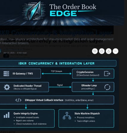
Connecting a C++ trading engine to Interactive Brokers via EClientSocket and EWrapper introduces concurrency challenges. Placing compute-heavy quantitative routines inside EWrapper callbacks blocks the network thread, causing TCP input buffers to overflow and quotes to fall behind.
+-----------------------------------------------------------------------------------+
|                        IBKR CONCURRENCY & INTEGRATION LAYER                       |
+-----------------------------------------------------------------------------------+
|                                                                                   |
|  +--------------------+         TCP Stream         +---------------------------+  |
|  | IB Gateway / TWS   | <========================> | CryptoSession             |  |
|  +--------------------+                            | (EClientSocket Outbound)  |  |
|                                                    +---------------------------+  |
|                                                                  |                |
|                                                                  v                |
|  +-------------------------------------+        Signal     +-------------------+  |
|  | Dedicated Reader Thread             | ----------------> | EReader Loop      |  |
|  | (Blocks on EReaderSignal)           |                   | processMsgs()     |  |
|  +-------------------------------------+                   +-------------------+  |
|                                                                  |                |
|                                                                  v                |
|  +-----------------------------------------------------------------------------+  |
|  | EWrapper Virtual Callback Interface (tickPrice, orderStatus, error)         |  |
|  +-----------------------------------------------------------------------------+  |
|            |                                                 |                    |
|            v                                                 v                    |
|  [Quote Integrity Engine]                         [State Machine Dispatch]        |
|  - Invalidate crossed books                       - Process transitions           |
|  - Reject zero volume                             - Track inflight orders         |
|  - Check monotonic clock staleness                                                |
|                                                                                   |
+-----------------------------------------------------------------------------------+
The Dual-Thread Reader Harness
The broker integration runs an independent OS thread to handle socket reads. The reader thread blocks on an EReaderSignal primitive, waking up only when the operating system receives a packet from TWS.
// ============================================================================
// PSEUDOCODE: DEDICATED EREADER THREAD EXECUTION LOOP
// Reference Implementation: CryptoSession.hpp
// Guide: https://hftcode.com/products/bitcoin-futures-volatility-analytics-ibkr-integration-c-17-technical-guide-code-architecture-pdf
// ============================================================================

PROCESS DedicatedReaderThread(ib_reader_ptr, ib_signal_ptr, system_running_flag)
    INPUT:
        ib_reader_ptr       : POINTER TO EReader
        ib_signal_ptr       : POINTER TO EReaderSignal
        system_running_flag : ATOMIC BOOLEAN

    WHILE system_running_flag == TRUE DO
        // Wait on OS-level condition variable until TCP data is present
        ib_signal_ptr->waitForSignal()

        // Decode incoming buffer and route directly to EWrapper callbacks
        ib_reader_ptr->processMsgs()
    END WHILE

    LOG_INFO("Reader thread terminated cleanly.")
END PROCESS
Quote Integrity Engine: Monotonic Clock Validation
Before updating local books or triggering orders from a quote, the quote must pass validation checks. These discard corrupted packets, inverted bid-ask spreads, and quotes delayed in network buffers.
// ============================================================================
// PSEUDOCODE: REAL-TIME QUOTE INTEGRITY ENGINE
// Reference Implementation: CryptoSession.hpp
// Guide: https://hftcode.com/products/bitcoin-futures-volatility-analytics-ibkr-integration-c-17-technical-guide-code-architecture-pdf
// ============================================================================

FUNCTION ValidateMarketDataQuote(bid_price, ask_price, bid_size, ask_size,
                                 packet_timestamp, max_allowable_staleness_ms)
    INPUT:
        bid_price, ask_price         : REAL
        bid_size, ask_size           : INT
        packet_timestamp             : INT64   // Timestamp provided in update
        max_allowable_staleness_ms   : INT64   // e.g., 200 ms maximum latency
    OUTPUT:
        is_quote_actionable          : BOOLEAN

    // Check 1: Positive prices
    IF bid_price <= 0.0 OR ask_price <= 0.0 THEN
        LOG_DEBUG("Quote Invalid: Non-positive price quote detected.")
        RETURN FALSE
    END IF

    // Check 2: Reject inverted / crossed books
    IF bid_price >= ask_price THEN
        LOG_WARNING("Quote Invalid: Crossed or locked book detected (Bid >= Ask).")
        RETURN FALSE
    END IF

    // Check 3: Zero volume liquidity check
    IF bid_size <= 0 OR ask_size <= 0 THEN
        LOG_DEBUG("Quote Invalid: Depth is zero on one or both sides.")
        RETURN FALSE
    END IF

    // Check 4: Monotonic staleness check
    current_monotonic_time <- GET_SYSTEM_STEADY_CLOCK_MILLISECONDS()
    elapsed_staleness <- current_monotonic_time - packet_timestamp

    IF elapsed_staleness > max_allowable_staleness_ms THEN
        LOG_WARNING("Quote Invalid: Stale quote dropped. Age: " + elapsed_staleness + "ms")
        RETURN FALSE
    END IF

    RETURN TRUE
END FUNCTION
Market Data Modes
Interactive Brokers supports four distinct market data modes via reqMarketDataType():
Mode 1 (Real-Time Live): Full streaming live data.
Mode 2 (Frozen): Displays the last recorded price after the market has closed.
Mode 3 (Delayed): Delayed by 15 minutes if real-time subscriptions are missing.
Mode 4 (Delayed-Frozen): Delayed quotes with post-market frozen values.
If an account credential lacks active CME market data subscriptions, IBKR can fall back to Mode 3 without failing explicitly. The execution harness must assert that the incoming mode is strictly Mode 1 during initialization, halting execution if delayed data is detected.
4. Deterministic Order Lifecycle, Execution Gates & Fault Recovery
When managing CME Bitcoin futures, order state tracking must be deterministic. The system cannot rely on assumptions; it must track every order through an explicit state machine that handles unacknowledged states and network disruptions.
       +-----------------------+
       |        CREATED        |
       +-----------------------+
                   |
                   | Pre-Trade Risk Validated
                   v
       +-----------------------+
       |       VALIDATED       |
       +-----------------------+
                   |
                   | Serialized to EClientSocket
                   v
       +-----------------------+
       |       SUBMITTED       |
       +-----------------------+
                   |
                   | IBKR Order ID Acknowledged
                   v
       +-----------------------+
       |     ACKNOWLEDGED      | <-----------------------+
       +-----------------------+                         |
         |         |         |                           | Partial
         |         |         | Partial Fill Received     | Fill
         |         |         +---------------------------+
         |         |
         |         +-------------------------+
         |                                   |
         | Complete Fill                     | Exchange Cancellation
         v                                   v
+-----------------+                 +-----------------+
|     FILLED      |                 |    CANCELLED    |
+-----------------+                 +-----------------+
         |                                   |
         +-----------------+-----------------+
                           |
                           | Socket Disconnect (Errors 1100 / 1101)
                           v
                +---------------------+
                |      UNCERTAIN      |  <-- Automated Trading Halted
                +---------------------+
The Six-State Execution Engine
CREATED: Allocated in memory with local risk limits verified.
VALIDATED: Passed discrete tick checks, margin buffers, and notional ceilings.
SUBMITTED: Transmitted over the network to TWS via
placeOrder().ACKNOWLEDGED: Confirmed by the CME matching engine with an assigned broker order ID.
FILLED / CANCELLED: Terminal states.
UNCERTAIN: Connection drops or timeouts occur while the order is inflight.
Disconnection Management: Errors 1100, 1101, and 1102
The EWrapper::error() method intercepts infrastructure messages from IBKR:
Error 1100: Connectivity between IB and TWS is lost.
Error 1101: Connectivity is restored, but data was lost while offline.
Error 1102: Connectivity is restored with no data loss (buffered data replayed).
// ============================================================================
// PSEUDOCODE: BROKER DISCONNECT AND ERROR EVENT HANDLER
// Reference Implementation: CryptoSession.hpp
// Guide: https://hftcode.com/products/bitcoin-futures-volatility-analytics-ibkr-integration-c-17-technical-guide-code-architecture-pdf
// ============================================================================

PROCESS HandleBrokerErrorEvents(error_code, error_message, order_state_machine, risk_controller)
    INPUT:
        error_code          : INT
        error_message       : STRING
        order_state_machine : INSTANCE OF OrderStateMachine
        risk_controller     : INSTANCE OF PreTradeRiskController

    MATCH error_code WITH
        CASE 1100:
            // Immediate kill-switch: Socket severed
            LOG_CRITICAL("IBKR Error 1100: Central connection severed. Halting quoting engine.")
            risk_controller.SetGlobalTradingHalt(TRUE)
            order_state_machine.TransitionAllActiveToUncertain()

        CASE 1101:
            // Connection restored with unrecoverable data loss
            LOG_CRITICAL("IBKR Error 1101: Connection restored with DATA LOSS. Full state audit required.")
            risk_controller.SetGlobalTradingHalt(TRUE)
            EXECUTE RunPositionAndOrderReconciliation(order_state_machine)

        CASE 1102:
            // Connection restored with full buffered stream
            LOG_INFO("IBKR Error 1102: Connection restored without data loss. Verifying book state.")
            order_state_machine.AuditSynchronizedFeeds()

        CASE 201:
            // CME matching engine rejected order
            LOG_WARNING("Exchange Order Rejection: " + error_message)
            order_state_machine.ProcessTerminalRejection(error_message)

        DEFAULT:
            LOG_DEBUG("Standard API Message [" + error_code + "]: " + error_message)
    END MATCH
END PROCESS
Position and Order Reconciliation
Following an unexpected disconnect or system restart, the engine audits its internal tracking ledger against the broker’s clearing ledger before resuming automated operations.
// ============================================================================
// PSEUDOCODE: POST-OUTAGE RECONCILIATION ENGINE
// Reference Implementation: Section 4 Order Lifecycle & Session Recovery
// Guide: https://hftcode.com/products/bitcoin-futures-volatility-analytics-ibkr-integration-c-17-technical-guide-code-architecture-pdf
// ============================================================================

FUNCTION RunPositionAndOrderReconciliation(client_socket, internal_ledger)
    INPUT:
        client_socket   : INSTANCE OF EClientSocket
        internal_ledger : INSTANCE OF LocalOrderDatabase
    OUTPUT:
        audit_passed    : BOOLEAN

    LOG_INFO("Commencing institutional state reconciliation...")

    // Step 1: Query broker for active order state
    client_socket.reqAllOpenOrders()
    broker_active_orders <- AWAIT_SYNCHRONOUS_REPLY(TIMEOUT_MS = 5000)

    // Step 2: Query broker for cleared position holdings
    client_socket.reqPositions()
    broker_positions <- AWAIT_SYNCHRONOUS_REPLY(TIMEOUT_MS = 5000)

    // Step 3: Match inflight local orders against broker state
    FOR EACH local_order IN internal_ledger.GetTrackedOrders() DO
        remote_order <- broker_active_orders.FindById(local_order.broker_id)

        IF remote_order == NULL THEN
            // If the order is missing from the active book, it was either filled or cancelled while offline
            LOG_WARNING("Order ID " + local_order.broker_id + " not found on active book. Querying execution reports.")
            local_order.SetState(UNCERTAIN)
        ELSE
            IF local_order.filled_shares != remote_order.filled_shares THEN
                LOG_INFO("Reconciling fill discrepancy for Order ID: " + local_order.broker_id)
                local_order.UpdateFilledShares(remote_order.filled_shares)
            END IF
        END IF
    END FOR

    // Step 4: Validate portfolio-level delta matches
    FOR EACH broker_pos IN broker_positions DO
        local_pos <- internal_ledger.GetContractPosition(broker_pos.contract_symbol)

        IF local_pos.net_position != broker_pos.position_amount THEN
            LOG_CRITICAL("CRITICAL ERROR: Portfolio delta mismatch! Local: "
                         + local_pos.net_position + " | Remote: " + broker_pos.position_amount)
            RETURN FALSE // Require human intervention
        END IF
    END FOR

    LOG_INFO("Reconciliation passed. System synchronized with broker ledger.")
    RETURN TRUE
END FUNCTION
5. Basis Term Structure, Calendar Spreads, and Legging Risk
Trading CME Bitcoin futures often involves calendar basis trading: capturing the annualized spread between front-month and back-month contracts.
+---------------------------------------------------------------------------------+
|                       CALENDAR BASIS EXECUTION PIPELINE                         |
+---------------------------------------------------------------------------------+
|                                                                                 |
|  [Front-Month Contract MBT_1] --------------+                                   |
|                                             |                                   |
|                                             v                                   |
|  [Back-Month Contract MBT_2]  -------> [Basis Engine]                           |
|                                             |                                   |
|                                             v                                   |
|                                   Compute Basis Metric:                         |
|                                   Annualized Return / Yield                     |
|                                             |                                   |
|                                             v                                   |
|                                   Threshold Evaluation:                         |
|                                   Exceeds Arbitrage Hurdle?                     |
|                                      /              \                           |
|                                    YES               NO                         |
|                                    /                  \                         |
|                                   v                    v                        |
|                        [Route Multi-Leg]          [Do Nothing]                  |
|                        [Spread Order   ]                                        |
|                                                                                 |
+---------------------------------------------------------------------------------+
Basis Calculations (Discrete vs. Continuous)
Given a front contract FnearF_{\text{near}}Fnear with time to maturity TnearT_{\text{near}}Tnear and a back contract FfarF_{\text{far}}Ffar with time to maturity TfarT_{\text{far}}Tfar, the annualized basis yield is computed under either simple or continuous compounding conventions:
// ============================================================================
// PSEUDOCODE: ANNUALIZED FUTURES BASIS CALCULATOR
// Reference Implementation: CryptoAnalytics.hpp
// Guide: https://hftcode.com/products/bitcoin-futures-volatility-analytics-ibkr-integration-c-17-technical-guide-code-architecture-pdf
// ============================================================================

FUNCTION ComputeAnnualizedBasis(price_near, expiry_near, price_far, expiry_far, continuous_flag)
    INPUT:
        price_near      : REAL    // Near-month futures price (F_1)
        expiry_near     : REAL    // Time to near expiry in years (T_1)
        price_far       : REAL    // Far-month futures price (F_2)
        expiry_far      : REAL    // Time to far expiry in years (T_2)
        continuous_flag : BOOLEAN // Toggle continuous vs. simple compounding
    OUTPUT:
        annualized_yield: REAL

    delta_time <- expiry_far - expiry_near

    IF delta_time <= 0.0 OR price_near <= 0.0 OR price_far <= 0.0 THEN
        RETURN 0.0
    END IF

    IF continuous_flag == TRUE THEN
        // Continuous compounding formulation: b = ln(F_far / F_near) / (T_far - T_near)
        annualized_yield <- LOG_NATURAL(price_far / price_near) / delta_time
    ELSE
        // Simple compounding formulation: b = ((F_far - F_near) / F_near) * (1 / delta_time)
        annualized_yield <- ((price_far - price_near) / price_near) * (1.0 / delta_time)
    END IF

    RETURN annualized_yield
END FUNCTION
Mitigating Legging Risk
When executing a synthetic calendar spread (buying the back month and selling the front month as separate orders), the system is vulnerable to legging risk: the front leg fills, the market moves sharply, and the back leg cannot be filled at the planned spread price.
The execution engine addresses this in one of two ways:
Exchange-Native Spread Instruments (
BAG/ Combos): IBKR supports CME native calendar spread instruments. By transmitting a multi-leg combo order, CME’s matching engine guarantees that both legs execute simultaneously or not at all.Aggressive Legging Strategy: If executing synthetically across fragmented order books, the first leg is posted as a passive limit order. Once filled, the second leg is dispatched immediately as an aggressive marketable limit order to close the basis delta.
// ============================================================================
// PSEUDOCODE: SYNTHETIC CALENDAR SPREAD LEGGING ENGINE
// Reference Implementation: Section 2 & Section 5 Execution Logic
// Guide: https://hftcode.com/products/bitcoin-futures-volatility-analytics-ibkr-integration-c-17-technical-guide-code-architecture-pdf
// ============================================================================

PROCESS ExecuteSyntheticCalendarSpread(contract_near, contract_far,
                                       target_spread_price, target_quantity,
                                       tick_size, max_slippage_ticks)
    INPUT:
        contract_near, contract_far : STRUCT // Contract definitions
        target_spread_price         : REAL
        target_quantity             : INT
        tick_size                   : REAL
        max_slippage_ticks          : INT

    // Phase 1: Post passive leg on the near-month contract
    passive_order <- CreateOrder(BUY, contract_near, target_quantity, PASSIVE_POST_ONLY)
    DispatchToSocket(passive_order)

    AWAIT_ORDER_FILL(passive_order, TIMEOUT_SECONDS = 15)

    IF passive_order.filled_quantity == 0 THEN
        CancelOrder(passive_order)
        LOG_INFO("Passive leg unfilled. Terminating spread execution with zero exposure.")
        RETURN
    END IF

    // Phase 2: Complete the aggressive hedge on the far-month contract
    actual_near_price <- passive_order.average_fill_price
    required_far_price <- actual_near_price + target_spread_price

    // Calculate maximum allowable limit price with slippage protection
    slippage_allowance <- max_slippage_ticks * tick_size
    aggressive_limit <- required_far_price + slippage_allowance

    hedge_order <- CreateOrder(SELL, contract_far, passive_order.filled_quantity,
                               SnapToValidTick(aggressive_limit, tick_size, SELL_SIDE))

    // Dispatch immediately as an aggressive marketable order
    DispatchToSocket(hedge_order)
    AWAIT_ORDER_FILL(hedge_order, TIMEOUT_SECONDS = 3)

    IF hedge_order.filled_quantity < passive_order.filled_quantity THEN
        LOG_CRITICAL("LEGGING FAILURE DETECTED: Partial fill on back leg! Directional delta unhedged.")
        TriggerEmergencyNeutralization(contract_far, passive_order.filled_quantity - hedge_order.filled_quantity)
    END IF
END PROCESS
6. Structural Payoffs and Monte Carlo Simulation
The final layer of the architecture focuses on quantitative valuation of volatility-linked notes and structured variance payoffs. Using the calculated realized variance and implied volatility surfaces, the Monte Carlo pricing engine simulates price paths for non-linear structures.
// ============================================================================
// PSEUDOCODE: MONTE CARLO PRICING FOR VARIANCE-LINKED STRUCTURES
// Reference Implementation: Section 5 Structured Payoff Engine
// Guide: https://hftcode.com/products/bitcoin-futures-volatility-analytics-ibkr-integration-c-17-technical-guide-code-architecture-pdf
// ============================================================================

FUNCTION PriceVarianceLinkedNote(spot_futures_price, risk_free_rate,
                                 base_volatility, time_to_maturity,
                                 num_paths, num_time_steps, variance_strike)
    INPUT:
        spot_futures_price : REAL
        risk_free_rate     : REAL
        base_volatility    : REAL
        time_to_maturity   : REAL
        num_paths          : INT  // e.g., 50,000 paths
        num_time_steps     : INT  // e.g., 252 daily steps
        variance_strike    : REAL // Target strike level (sigma_k^2)
    OUTPUT:
        fair_present_value : REAL

    dt <- time_to_maturity / num_time_steps
    sqrt_dt <- SQUARE_ROOT(dt)
    drift <- (risk_free_rate - (0.5 * base_volatility * base_volatility)) * dt
    diffusion_scalar <- base_volatility * sqrt_dt

    discount_factor <- EXPONENTIAL(-risk_free_rate * time_to_maturity)
    accumulated_payoff <- 0.0

    FOR path FROM 1 TO num_paths DO
        current_path_price <- spot_futures_price
        sum_sq_returns <- 0.0

        FOR step FROM 1 TO num_time_steps DO
            // Sample standard normal Gaussian variate
            epsilon <- GENERATE_GAUSSIAN_RANDOM_VARIABLE(mean = 0.0, stdev = 1.0)

            // Advance geometric Brownian motion step
            next_path_price <- current_path_price * EXPONENTIAL(drift + (diffusion_scalar * epsilon))

            // Calculate step log return
            log_ret <- LOG_NATURAL(next_path_price / current_path_price)
            sum_sq_returns <- sum_sq_returns + (log_ret * log_ret)

            current_path_price <- next_path_price
        END FOR

        // Calculate realized variance for this trajectory
        path_realized_variance <- (sum_sq_returns / time_to_maturity)

        // Structured payoff: max(0, Realized Variance - Variance Strike)
        terminal_payoff <- MAXIMUM(0.0, path_realized_variance - variance_strike)
        accumulated_payoff <- accumulated_payoff + terminal_payoff
    END FOR

    fair_present_value <- discount_factor * (accumulated_payoff / num_paths)
    RETURN fair_present_value
END FUNCTION
7. Comparative Architectural Review
+---------------------------------------------------------------------------------------------------------+
|                                    TRADING SYSTEM DESIGN COMPARISON                                     |
+--------------------------+--------------------------------------+---------------------------------------+
| Architectural Domain     | Generic Python/Research Stack        | HFTCODE C++17 Reference Design        |
+--------------------------+--------------------------------------+---------------------------------------+
| Language & Runtime       | Interpreted Python / GIL constraints | Native ISO C++17; zero third-party    |
|                          | with garbage collection pauses       | math bloat (std:: only)               |
| Numerical Precision      | Floating-point continuous midpoints  | Integer-tick snapping with passive    |
|                          | causing exchange rejections          | limit execution constraints           |
| Broker Integration       | Blocking HTTP REST/Polling loops     | Multi-threaded socket reader harness  |
|                          | vulnerable to missed messages        | on IBKR EClientSocket / EWrapper      |
| Quote Validation         | Assumes incoming data is clean       | Real-time validation: rejects crossed |
|                          | and in sequence                      | books, zero depth, and stale timestamps|
| Volatility Modeling      | Unbounded Newton-Raphson solvers     | Numerically bounded bisection solvers |
|                          | prone to divergence when Vega -> 0   | with strict convergence guarantees    |
| Recovery Mechanics       | Naive binary states (Pending/Filled) | Six-state non-blocking state machine   |
|                          | vulnerable to network disconnects    | with automated error-code recovery    |
+--------------------------+--------------------------------------+---------------------------------------+
Implementation Takeaways
Moving algorithmic derivative models into production requires shifting focus from pure statistics to execution engineering:
Exchange Rules Dictate System Logic: Mathematical models must respect the physical constraints of the venue—discrete tick boundaries, integer multipliers, and dynamic margin requirements.
Deterministic Root-Finding: When calculating implied volatility in production, bounded convergence algorithms (such as bisection) provide stability where faster methods like Newton-Raphson risk diverging on edge cases.
Decoupled Network Architecture: Processing analytics within network callback threads degrades socket throughput. An execution harness should isolate socket ingestion from calculation routines.
State Machine Completeness: An order state machine must explicitly handle ambiguous and disconnected states, maintaining pre-trade gates and automated reconciliation routines to protect capital when connectivity drops.
Accessing the Full Source Code & Architecture Document
The algorithms and execution architectures discussed in this article are available in full inside the technical guide:
Direct Access: Bitcoin Futures, Volatility Analytics & IBKR Integration — C++17 Technical Guide & Code Architecture (PDF)
Code Artifacts Included: Full source code for
CryptoAnalytics.hpp(pricing, Greeks, realized volatility, bisection solvers) andCryptoSession.hpp(Interactive BrokersEWrapper/EClientSocketintegration, quote validation, and state machine recovery).